4.1 Vector Fields
Definition 4.1.1. Let \(D\) be a set in \(\mathbb {R}^2\) ( a plane region). A vector field on \(\mathbb {R}^2\) is a function \(F\) that assigns to each point \((x,y)\) in \(D\) a two dimensional vector \(F(x,y)\).
\(F(x,y)\) can be written in terms of its component functions \(P\) and \(Q\) as follows: \[F(x,y) = P(x,y)\textbf {i} + Q(x,y)\textbf {j}\hspace {0.4cm} \text {or}\hspace {0.4cm} F = P\textbf {i} + Q\textbf {j}\] \(P\) and \(Q\) are scalar functions and sometimes called scalar fields.
Definition 4.1.2. Let \(E\) be a subset of \(\mathbb {R}^3\). A vector field on \(\mathbb {R}^3\) is a function \(F\) that assigns to each point \((x,y,z)\) in \(E\) a three-dimensional vector \(F(x,y,z)\). \(F\) is continuous if and only if its component functions \(P\) , \(Q\) and \(R\) are continuous.
Example 4.1.3. A vector field on \(\mathbb {R}^2\) is defined by \(F(x,y) = -y\textbf {i} + x\textbf {j}\). Describe \(F\) by sketching some of the vectors.
\[F(1,0) = \textbf {j},\hspace {0.5cm} F(0,1) = \textbf {i},\hspace {0.5cm} F(-1,0) = -\textbf {j},\hspace {0.5cm} F(0,-1) = \textbf {i}, \hspace {0.5cm} F(-1,-1) = \textbf {i}-\textbf {j},\hspace {0.5cm} F(1,1) = -\textbf {i} + \textbf {j}\]
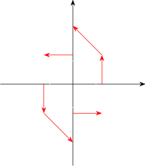
It appears that each arrow is tangent to a circle with centre at the origin.
Example 4.1.4. Imagine a fluid flowing steadily along a pipe and let \(V(x,y,z)\) be the velocity vector at a point \((x,y,z)\). Then \(V\) assigns a vector to each point \((x,y,z)\) in a certain domain \(E\) the interior of the pipe and so \(V\) is a vector field on \(\mathbb {R}^3\) called a velocity field. Velocity fields occur in other areas of physics. For instance the vector field in example 1 could be used as the velocity field describing the counter-clockwise movement of a wheel.
Questions on this section
Stuck on something here? Ask below and it stays attached to this topic.