3 Multiple Integration

The definite integral of one variable adds up a quantity along an interval. The multiple integral does the same over a region of the plane or of space, and the construction is the same in every case: cut the region into small pieces, multiply the value of the function on each piece by its area or volume, add, and pass to the limit.

The practical content of the section is that such an integral can be evaluated as a succession of ordinary single integrals. That is Fubini’s theorem, and it is what makes the subject computable rather than merely definable. The work then becomes a matter of describing the region correctly and choosing the order of integration well, which is why so much attention goes to regions of Type I and Type II and to reversing the order.

Polar, cylindrical and spherical coordinates follow, each earning its place by turning a region with an awkward boundary into a rectangle. The change of variables formula unifies them: the Jacobian of the previous section reappears as the factor by which the change of coordinates stretches area or volume, and it is exactly what must be inserted to keep the answer right.

The section closes with the applications the machinery was built for — volume, mass, centre of mass, moments of inertia and surface area.

Recall the single-variable construction. For \(f\geq 0\) on \([a,b]\), divide the interval into \(n\) subintervals of width \(\Delta x\), choose a sample point \(x_i^*\) in each, and approximate the area under the curve by rectangles.

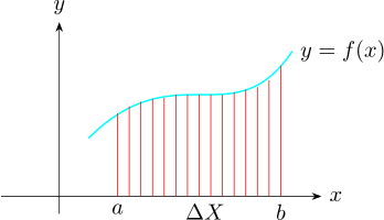
The area under the curve is the limit of the Riemann sums, \[\int ^b_a f(x)\,dx = \lim _{n\to \infty }\sum ^{n}_{i=1} f(x_i^*)\, \Delta x ,\] each term being the area of one approximating rectangle.

Questions on this section

Stuck on something here? Ask below and it stays attached to this topic.