1.5 Measures Of Central Tendencies
Central tendency: of a distribution is an estimate of the ”centre” of a distribution of values.
There are three major types of estimates of central tendency
- 1.
- Mean
- 2.
- Median
- 3.
- Mode
1.5.1 Mean
The mean is probably the most commonly used method of describing central tendency.
Definition 1.17. The mean is the central value of the given observation. \begin {align*} &\textbf {Notation}\\ \sum \hspace {0.3cm}&-\hspace {0.3cm}\text {Sum}\\\ \overline {X}\hspace {0.3cm}&-\hspace {0.3cm}\text {Mean}\\ n\hspace {0.3cm}&-\hspace {0.3cm}\text {Number of observations} \end {align*}
\[\overline {X}=\frac {1}{n}\sum _1^nX\hspace {1cm}\text {Ungrouped Data}\]
The mean is determined by summing all the observations and dividing by the number of
observations.
Solution. \[\overline {X}=\frac {1}{n}\sum _{i=1}^{5}X_i=\frac {0+5+2+3+5}{5}=\frac {15}{5}=3.\]
For data already summarised in a frequency table, each value is weighted by how often it occurs: \[\overline {X}=\frac {\sum fX}{\sum f}.\]
Solution. Add an \(fX\) row and total both:
| \(X\) | 0 | 1 | 2 | 3 | Total |
| \(f\) | 3 | 2 | 2 | 1 | 8 |
| \(fX\) | 0 | 2 | 4 | 3 | 9 |
\[\overline {X}=\frac {\sum fX}{\sum f}=\frac {9}{8}=1.125.\]
When the data have been grouped into classes the individual values are no longer available, so each observation is represented by the mid-point of its class.
Example 1.20. Estimate the mean of the grouped data below.
| Class interval | \(1\)–\(5\) | \(6\)–\(10\) | \(11\)–\(15\) | \(16\)–\(20\) |
| \(f\) | 1 | 3 | 2 | 1 |
Solution. The mid-point of a class is the average of its two limits: for \(1\)–\(5\) that is \((1+5)/2=3\), and so on.
| Class interval | Mid-point \(X\) | \(f\) | \(fX\) |
| \(1\)–\(5\) | 3 | 1 | 3 |
| \(6\)–\(10\) | 8 | 3 | 24 |
| \(11\)–\(15\) | 13 | 2 | 26 |
| \(16\)–\(20\) | 18 | 1 | 18 |
| Total | 7 | 71 |
\[\overline {X}=\frac {\sum fX}{\sum f}=\frac {71}{7}=10.14.\]
Example 1.21. Calculate the mean for each of the following sets of data.
- (a).
- The raw values \(15,\ 20,\ 21,\ 20,\ 36,\ 15,\ 25,\ 15\).
- (b).
- Data summarised in a frequency table:
\(X\) 0 1 2 3 4 5 \(f\) 3 5 3 2 1 1 - (c).
- Data grouped into classes:
Class interval \(1\)–\(5\) \(6\)–\(10\) \(11\)–\(15\) \(16\)–\(20\) \(21\)–\(25\) \(26\)–\(30\) \(31\)–\(35\) \(f\) 1 3 5 4 2 2 1
Solution. The three parts are the same calculation at three levels of summary, and each level costs a little accuracy.
(a). Raw values. Every observation is present, so the mean is exact: \[\overline {X}=\frac {1}{n}\sum X=\frac {15+20+21+20+36+15+25+15}{8}=\frac {167}{8}=20.875.\]
(b). Frequency table. The individual values are still known; they have only been counted rather than listed. Multiply each value by how often it occurs:
| \(X\) | 0 | 1 | 2 | 3 | 4 | 5 | Total |
| \(f\) | 3 | 5 | 3 | 2 | 1 | 1 | 15 |
| \(fX\) | 0 | 5 | 6 | 6 | 4 | 5 | 26 |
\[\overline {X}=\frac {\sum fX}{\sum f}=\frac {26}{15}=1.733.\] This is still exact – writing \(2\) three times or writing “\(2\), three times” is the same information.
(c). Grouped data. Here the individual values are gone. All we know is how many fell in each class, so each observation is taken to sit at its class mid-point:
| Class interval | Mid-point \(X\) | \(f\) | \(fX\) |
| \(1\)–\(5\) | 3 | 1 | 3 |
| \(6\)–\(10\) | 8 | 3 | 24 |
| \(11\)–\(15\) | 13 | 5 | 65 |
| \(16\)–\(20\) | 18 | 4 | 72 |
| \(21\)–\(25\) | 23 | 2 | 46 |
| \(26\)–\(30\) | 28 | 2 | 56 |
| \(31\)–\(35\) | 33 | 1 | 33 |
| Total | 18 | 299 |
\[\overline {X}=\frac {\sum fX}{\sum f}=\frac {299}{18}=16.61.\]
This last answer is an estimate, not the mean of the original data. Treating every observation in \(11\)–\(15\) as though it were exactly \(13\) is only right on average, and the error does not necessarily cancel. Once data have been grouped, the exact mean cannot be recovered – which is worth remembering before grouping data you still need to work with.
1.5.2 Median and Interquartile Range
The median is the value found on the middle of the set of the ordered observations.
One way to compute the median is to list all scores in numerical order, and locate the score on the
middles of the observation.
When you order the observations \(n\) can either be odd or even
- 1.
- if \(n\) is odd, then the median is one of the observations.
- 2.
- if \(n\) is even, the median is not one of the observation.
Example 1.22. Find the median of each of the following.
- (a)
- The eight observations \(15,\; 20,\; 21,\; 20,\; 36,\; 15,\; 25,\; 15\).
- (b)
- The ungrouped frequency distribution in Table (b).
- (c)
- The grouped frequency distribution in Table (c).
| \(X\) | 0 | 1 | 2 | 3 | 4 | 5 |
| \(f\) | 3 | 5 | 3 | 2 | 1 | 1 |
Solution. (a) Order the values first. Nothing about a median means anything until you do. \[15,\; 15,\; 15,\; 20,\; 20,\; 21,\; 25,\; 36\] There are \(n=8\) observations. Since \(n\) is even the median is not one of them; it is the average of the \(4^{\text {th}}\) and \(5^{\text {th}}\) values: \[\text {Median}=\frac {20+20}{2}=20\]
(b) Add a cumulative frequency column.
| \(X\) | \(f\) | \(Cf\) |
| 0 | 3 | 3 |
| 1 | 5 | 8 |
| 2 | 3 | 11 |
| 3 | 2 | 13 |
| 4 | 1 | 14 |
| 5 | 1 | 15 |
| Total | 15 | |
Here \(n=\sum f=15\), which is odd, so the median is one of the observations: the \(\tfrac {1}{2}(n+1)=8^{\text {th}}\) value. Reading down the \(Cf\) column, the count first reaches \(8\) at \(X=1\), so \[\text {Median}=1\]
(c) The individual values are gone, so the median can no longer be read off a list — it has to be located inside a class.
| Class Interval | \(f\) | \(Cf\) | Lower boundary |
| \(1-5\) | 1 | 1 | 0.5 |
| \(6-10\) | 3 | 4 | 5.5 |
| \(11-15\) | 5 | 9 | 10.5 |
| \(16-20\) | 4 | 13 | 15.5 |
| \(21-25\) | 2 | 15 | 20.5 |
| \(26-30\) | 2 | 17 | 25.5 |
| \(31-35\) | 1 | 18 | 30.5 |
| Total | 18 | ||
Here \(n=18\), so \(\tfrac {n}{2}=9\). The class median is the first class whose cumulative frequency reaches \(9\), which is \(11-15\). For that class \[L_m=10.5,\hspace {0.8cm} F=4,\hspace {0.8cm} f_m=5,\hspace {0.8cm} i=5\] and the formula set out in the next subsection gives \[\text {Median}=L_m+\Bigg (\frac {\frac {n}{2}-F}{f_m}\Bigg )i =10.5+\Bigg (\frac {9-4}{5}\Bigg )5=15.5\]
The answer lands exactly on the upper boundary of the class, which looks odd but is correct here: the cumulative frequency reaches \(\tfrac {n}{2}=9\) precisely at the end of the class \(11-15\), so the interpolation runs the whole way across it. Notice also that the classes are written \(1-5\), \(6-10\) and so on, yet the boundaries used are \(0.5\), \(5.5\), \(10.5\). The gap between \(5\) and \(6\) is an artefact of recording whole numbers; the underlying scale is continuous, and it is the boundaries that the formula needs.
1.5.3 Median from a frequency table for discrete data
If data is not grouped the median can easily be found by arranging the data in order.
In the table below we can use the Cf to find the median.
| Score | \(f\) | Cf |
| 1 | 7 | 7 |
| 2 | 15 | 22 |
| 3 | 10 | 32 |
| 4 | 3 | 35 |
| 5 | 9 | 44 |
| 6 | 6 | 50 |
\(n=50\hspace {0.5cm}\implies \) Md = 25\(^{\text {th}}\) value and 26\(^{\text {th}}\) value = \(\frac {3+3}{2}=3\).
1.5.4 Median of a Continuous Data
| C.I | \(f\) | Cf | True Upper Class Limits |
| \(4.0-5.9\) | 1 | 1 | 5.95 |
| \(6.0-7.9\) | 3 | 4 | 7.95 |
| \(8.0-9.9\) | 7 | 11 | 9.95 |
| \(10.0-11.9\) | 9 | 20 | 11.95 |
| \(12.0-13.9\) | 9 | 29 | 13.95 |
| \(14.0-15.9\) | 12 | 41 | 15.95 |
| \(16.0-17.9\) | 8 | 49 | 17.95 |
| \(18.0-19.9\) | 1 | 50 | 19.95 |
If we assume the curve is linear between \(A\) and \(B\).
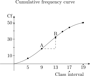
\(\frac {50}{2}=25^{\text {th}}\) value and \(26^{\text {th}}\) value.

Similar triangles give
\[\frac {AD}{AC}=\frac {ED}{BC} \hspace {0.8cm}\implies \hspace {0.8cm}\frac {m-11.95}{13.95-11.95}=\frac {25-20}{29-20}\]
\[\implies \hspace {0.5cm} m=11.95+\Bigg (\frac {5}{9}\Bigg )2=11.95+1.11=13.06\]
which is the grouped median formula again, read off the picture instead of quoted.
1.5.5 Median for grouped data
- Step 1:
- Construct the cumulative frequency distribution.
- Step 2:
- Decide the class that contain the median. Class Median is the first class with the value of cumulative frequency equal at least \(n/2\).
- Step 3:
- Find the median by using the following formula: \[\text {Median} = L_m + \Bigg (\frac {\frac {n}{2}-F}{f_m}\Bigg )\, i\]
Where:
- \(n = \) the total frequency
- \(F = \) the cumulative frequency before class median
- \(f_m = \) the frequency of the class median
- \(i = \) the class width
- \(L_m = \) the lower boundary of the class median
Example 1.23. Based on the grouped data below, find the median
| Time to travel | |
| to work | Frequency |
| \(1 - 10\) | 8 |
| \(11 - 20\) | 14 |
| \(21 - 30\) | 12 |
| \(31 - 40\) | 9 |
| \(41 - 50\) | 7 |
Solution. Step 1: Construct the cumulative frequency distribution.
| Time to travel | Cumulative | |
| to work | Frequency | Frequency |
| \(1 - 10\) | 8 | 8 |
| \(11 - 20\) | 14 | 22 |
| \(21 - 30\) | 12 | 34 |
| \(31 - 40\) | 9 | 43 |
| \(41 - 50\) | 7 | 50 |
\(\displaystyle {\frac {n}{2}=\frac {50}{2}=25}\implies \) Class median is the \(3^{\text {rd}}\) class.
So \(F=22,\hspace {0.2cm} f_m=12,\hspace {0.2cm} L_m=21.5\hspace {0.2cm}\) and \(\hspace {0.2cm}i=10\). Therefore
\begin {align*} \text {Median} & = L_m + \Bigg (\frac {\frac {n}{2}-F}{f_m}\Bigg )\, i\\\\ & = 21.5 + \Bigg (\frac {25-22}{12}\Bigg )\times 10\\ & = 24 \end {align*}
Thus, 25 persons take less than 24 minutes to travel to work and another 25 persons take more than
24 minutes to travel to work.
1.5.6 Quartiles for grouped data
Using the same method of calculation as in the median. We can get \(Q_1\) and \(Q_3\) equation as follows: \[Q_1 = L_{Q_1} + \Bigg (\frac {\frac {n}{4}- F}{f_{Q_1}}\Bigg ) \, i\]
\[Q_3 = L_{Q_3} + \Bigg (\frac {\frac {3n}{4}- F}{f_{Q_3}}\Bigg ) \, i\]
Example 1.24. Based on the grouped data below, find the interquartile range.
| Time to travel | |
| to work | Frequency |
| \(1 - 10\) | 8 |
| \(11 - 20\) | 14 |
| \(21 - 30\) | 12 |
| \(31 - 40\) | 9 |
| \(41 - 50\) | 7 |
Solution. Step 1: Construct the cumulative frequency distribution.
| Time to travel | Cumulative | |
| to work | Frequency | Frequency |
| \(1 - 10\) | 8 | 8 |
| \(11 - 20\) | 14 | 22 |
| \(21 - 30\) | 12 | 34 |
| \(31 - 40\) | 9 | 43 |
| \(41 - 50\) | 7 | 50 |
Step 2: Determine the \(Q_1\) and \(Q_3\)
Class \(\displaystyle {Q_1 = \frac {n}{4} = \frac {50}{4}=12.5}\implies \) Class \(Q_1\) is the \(2^{\text {nd}}\) class. Therefore, \begin {align*} Q_1 & = L_{Q_1} + \Bigg (\frac {\frac {n}{4}-F}{f_{Q_1}}\Bigg )\, i\\\\ & = 10.5 + \Bigg (\frac {12.5-8}{14}\Bigg )\times 10\\\\ \implies Q_1 & = 13.7143\\ \end {align*}
Class \(Q_3 = \displaystyle {\frac {3n}{4} = \frac {3(50)}{4} = 37.5} \implies \) Class \(Q_3\) is the \(4^{\text {th}}\) class. Therefore, \begin {align*} Q_3 & = L_{Q_3} + \Bigg (\frac {\frac {3n}{4}-F}{f_{Q_3}}\Bigg )\, i\\\\ & = 30.5 + \Bigg (\frac {37.5-34}{9}\Bigg )\times 10\\\\ \implies Q_3 & = 34.3889\\ \end {align*}
Interquartile Range: \(IQR = Q_3 - Q_1\)
Calculate the \(IQR\) \begin {align*} IQR & = Q_3 - Q_1\\ & = 34.3889 - 13.7143\\ & = 20.6746\\ \end {align*}
1.5.7 Mode
The mode is the most frequently occurring value in the data set.
If the data is not grouped the mode is simply the value that appears most. But if data is grouped in
C.I we call this as mode class.
Example 1.25. Find the mode of each of the following.
- (a).
- \(1,\ 2,\ 3,\ 4,\ 5\)
- (b).
- \(0,\ 1,\ 4,\ 0,\ 3,\ 0,\ 1,\ 7,\ 1,\ 9\)
- (c).
- the ungrouped distribution below.
- (d).
- the grouped distribution below.
Solution. (a). Every value occurs once, so no value occurs more often than the others and there is no mode. This is worth noticing: unlike the mean and the median, the mode need not exist.
(b). Both \(0\) and \(1\) occur three times, and nothing occurs more often, so there are two modes – \(0\) and \(1\). Such a distribution is called bimodal. Here too the mode differs from the other averages: it need not be unique.
(c). The largest frequency is \(7\), against \(X=0\), so the mode is 0.
(d). The data are grouped, so what can be identified is a modal class rather than a single modal value — the individual observations are no longer visible. The largest frequency is \(3\), and three classes share it: \[\textbf {modal classes: } 6-10,\ 11-15\ \text {and}\ 16-20.\] With three of the four classes tied, the mode tells us almost nothing here. That is the honest conclusion: an average that cannot distinguish three quarters of the data is the wrong summary for it, and the median or mean would serve better.
Remark 1.26. The mode is the only average that can be used with nominal data. There is no arithmetic mean of “Lusaka, Ndola, Ndola, Kitwe”, and no median either, since the categories have no order – but Ndola is plainly the most common, and that is the mode.
1.5.8 Mode for grouped data
- \(\bullet \)
- For grouped data, class mode (or modal class) is the class with the highest frequency.
- \(\bullet \)
- To find mode for grouped data, use the following formula:
\[\text {Mode} = L_{m_o} + \Bigg (\frac {\Delta 1}{\Delta 1 + \Delta _2}\Bigg )\, i\]
where:
- \(i\)
- is the class width
- \(\Delta _1\)
- is the difference between the frequency of class mode and the frequency of the class after the class mode.
- \(\Delta _2\)
- is the difference between the frequency of class mode and frequency of the class before the class mode.
- \(L_{m_0}\)
- is the lower boundary of class mode.
Example 1.27. Based on the grouped data below, find the mode.
| Time to travel | |
| to work | Frequency |
| \(1 - 10\) | 8 |
| \(11 - 20\) | 14 |
| \(21 - 30\) | 12 |
| \(31 - 40\) | 9 |
| \(41 - 50\) | 7 |
Solution. Based on the table \(L_{m_0} = 10.5\hspace {0.1cm},\hspace {0.2cm} \Delta _1 = (14-8)=6\hspace {0.1cm},\hspace {0.2cm}\Delta _2 = (14-12)=2\hspace {0.2cm}\) and \(\hspace {0.2cm} i = 10\)
\begin {align*} \text {Mode} & = 10.5 + \Bigg (\frac {6}{6 + 2}\Bigg )\times 10\\ & = 17.5\\ \end {align*}
Selecting among the mode, median and mean. The choice of the measure of central tendency depends
on the distribution of the data at hand.
If the data at hand is assumed to normally distributed \(N\thicksim (0,1)\) mean will give a true reflection of the data,
otherwise we consider the mode or median.
The first consideration is the type of data. If the variable is categorical, the mode is the single measure
that best describe the data.
The second consideration in selecting the index is to ask whether the total of all observation is of any
interest, if the answer is yes, then the mean is the proper index of the central tendency. If the total is
of no interest then depending on whether the histogram is symmetric on skewed one must use either
mean or median respectively.
In all cases the histogram must be unimodal.
Questions on this section
Stuck on something here? Ask below and it stays attached to this topic.