1.15 Moments
Four questions describe the shape of any distribution, and each is answered by a moment:
- 1st.
- Where is it? – the mean.
- 2nd.
- How spread out is it? – the variance.
- 3rd.
- Is it lopsided, and which way? – the skewness.
- 4th.
- How heavy are the tails? – the kurtosis.
That is the whole idea. A moment is what you get by raising each deviation to a power and averaging; the power decides which question is answered. Higher powers give more weight to observations far from the centre, which is why the third and fourth moments say something about the tails while the first two do not.
1.15.1 Raw moments (about the origin)
Definition 1.44. The \(r\)th raw moment, taken about zero, is \[\mu '_r=\frac {\sum X^r}{n} \qquad \text {or, for a frequency distribution,}\qquad \mu '_r=\frac {\sum fX^r}{\sum f}.\]
The first raw moment is the mean: \[\mu '_1=\frac {\sum X}{n}=\overline {X}.\] (The zeroth is \(\mu '_0=1\), since \(X^0=1\) for every observation. It is worth stating once and then forgetting.)
1.15.2 Central moments (about the mean)
Raw moments answer the first question but not the others, because they are measured from zero, which is an arbitrary place. To describe shape we measure from the centre.
Definition 1.45. The \(r\)th central moment is \[\mu _r=\frac {\sum (X-\overline {X})^r}{n} \qquad \text {or}\qquad \mu _r=\frac {\sum f(X-\overline {X})^r}{\sum f}.\]
Take them in turn:
- \(\mu _1=\frac {\sum (X-\overline {X})}{n}=0\) always – the deviations from the mean cancel by definition. This is not a useless fact: it is the reason the second moment has to square them.
- \(\mu _2=\sigma ^2\), the variance.
- \(\mu _3\) measures lopsidedness. Cubing preserves sign, so observations far to the right contribute large positive amounts and those far to the left large negative ones. If the two sides balance, \(\mu _3=0\).
- \(\mu _4\) measures tail weight. The fourth power is large only for observations far from the mean, so \(\mu _4\) is dominated by the extremes.
1.15.3 Converting between them
Central moments are usually computed from raw ones, because \(\sum X^r\) is easier to accumulate than \(\sum (X-\overline {X})^r\): \[\mu _2=\mu '_2-\left (\mu '_1\right )^2,\] \[\mu _3=\mu '_3-3\mu '_2\mu '_1+2\left (\mu '_1\right )^3,\] \[\mu _4=\mu '_4-4\mu '_3\mu '_1+6\mu '_2\left (\mu '_1\right )^2-3\left (\mu '_1\right )^4.\] The first of these is the familiar \(\sigma ^2=\overline {X^2}-\overline {X}^2\). Note that the subtracted term is the raw first moment \(\mu '_1=\overline {X}\); the central first moment \(\mu _1\) is zero and would subtract nothing.
Where those three come from. They are not separate results to be memorised. Expand \((X-\overline {X})^r\) by the binomial theorem, remembering that \(\overline {X}=\mu '_1\) is a constant, and average term by term: \[\mu _r=\sum _{j=0}^{r}(-1)^j\binom {r}{j}\,\mu '_{r-j}\left (\mu '_1\right )^{j}.\] The alternating sign comes from the minus in \((X-\overline {X})\), and \(\binom {r}{j}\) is the ordinary binomial coefficient.
Taking \(r=0,1,2\) in turn, and using \(\mu '_0=1\): \begin {align*} \mu _0 &=\binom {0}{0}\mu '_0 &&=1\\[2pt] \mu _1 &=\binom {1}{0}\mu '_1-\binom {1}{1}\mu '_0\,\mu '_1 &&=\mu '_1-\mu '_1=0\\[2pt] \mu _2 &=\binom {2}{0}\mu '_2-\binom {2}{1}\mu '_1\,\mu '_1+\binom {2}{2}\mu '_0\left (\mu '_1\right )^2 &&=\mu '_2-2\left (\mu '_1\right )^2+\left (\mu '_1\right )^2\\ & &&=\mu '_2-\left (\mu '_1\right )^2 \end {align*}
and \(r=3\) and \(r=4\) give the third and fourth formulas above in the same way.
The first two are worth reading rather than passing over. \(\mu _0=1\) always, because averaging \((X-\overline {X})^0=1\) over \(n\) observations gives \(1\); it carries no information. And \(\mu _1=0\) always — the two terms cancel exactly. Neither depends on the data at all, which is why the useful moments start at \(\mu _2\).
1.15.4 Making them comparable
\(\mu _3\) has the cube of the original units and \(\mu _4\) the fourth power, so neither can be compared between data sets measured in different units – or even judged large or small on its own. Dividing by the appropriate power of \(\sigma \) removes the units entirely: \[\text {Skewness}=\frac {\mu _3}{\sigma ^3},\qquad \text {Kurtosis}=\frac {\mu _4}{\sigma ^4}.\] These are pure numbers, and can be read directly:
- Skewness \(>0\): the right tail is longer – the distribution leans left with a tail running right. Skewness \(<0\): the reverse. Skewness \(=0\): symmetric.
- Kurtosis \(=3\) for a normal distribution. Above 3 means heavier tails than normal (more extreme values than one would expect); below 3 means lighter. Because 3 is the reference, the excess kurtosis, \(\frac {\mu _4}{\sigma ^4}-3\), is often quoted instead, so that the normal sits at zero.
Example 1.46. Calculate \(\mu _1, \mu _2, \mu _3, \mu _4\) for the data given below
Direct Method
| \(X\) | \(X-\overline {X}\) | \((X-\overline {X})^2\) | \((X-\overline {X})^3\) | \((X-\overline {X}^4\) |
| 10 | \(-20\) | 400 | \(-8 000\) | 160, 000 |
| 20 | \(-10\) | 100 | \(-1 000\) | 10 000 |
| 30 | 0 | 0 | 0 | 0 |
| 40 | 10 | 100 | 1 000 | 10 000 |
| 50 | 20 | 400 | 8 000 | 160 000 |
| 150 | 0 | 1 000 | 0 | 340 000 |
Solution.
\[\overline {X}=\frac {1}{n}\sum X=\frac {1}{5}(150)\hspace {0.5cm}\implies \hspace {0.5cm}\overline {X}=30\]
\[\mu _1=\frac {\sum (X-\overline {X})}{n}=\frac {0}{5}=0\]
\[\mu _2=\frac {\sum (X-\overline {X})^2}{n}=\frac {1000}{5}=200\]
\[\mu _3=\frac {\sum (X-\overline {X})^3}{n}=\frac {0}{5}=0\]
\[\mu _4=\frac {\sum (X-\overline {X})^4}{n}=\frac {340,000}{5}=68, 000\]
Indirect Method
| \(X\) | \(D_X=X-a\) | \(D_X^2\) | \(D^3_X\) | \(D_X^4\) |
| 10 | \(-20\) | 400 | \(-8 000\) | 160, 000 |
| 20 | \(-10\) | 100 | \(-1 000\) | 10, 000 |
| 30 | 0 | 00 | 0 | 0 |
| 40 | 10 | 100 | 1 000 | 10, 000 |
| 50 | 20 | 400 | 8 000 | 160, 000 |
| 0 | 1 000 | 0 | 340,000 | |
\[\mu '_1=\frac {\sum D_X}{n},\hspace {0.8cm} \mu '_2=\frac {\sum D^2_X}{n},\hspace {0.8cm}\mu '_3=\frac {\sum D^3_X}{n},\hspace {0.8cm}\mu '_4=\frac {\sum D^4_X}{n}\]
\[\mu _1=0\hspace {0.5cm}\text {always}\]
\[\mu _2=\mu '_2-\left (\mu '_1\right )^2=\frac {1000}{5}-0^2=200\]
\[\mu _3=\mu '_3-3\mu '_2\mu '_1+2\mu ^{\prime 3}_1=0-3(200)(0)+2(0)^3=0\]
\[\mu _4=\mu '_4-4\mu '_3\mu '_1+6\mu '_2\mu ^{\prime 2}_1-3\mu ^{\prime 4}_1=68,000-4(0)(0)+6(200)(0)^2-3(0)^4=68,000\]
Note 1.47. The two methods gave identical numbers at every step, which makes the indirect method look pointless. That is only because \(a=30\) was chosen here, and \(30\) happens to be the mean, so every \(\mu '_r\) was already a central moment and each correction term collapsed to zero. Choose \(a\) anywhere else — as in the next example, where \(a=7\) but the mean is \(6.9\) — and the correction terms do real work.
1.15.5 Moment Ratios
\[\beta _1=\frac {\mu ^2_3}{\mu ^3_2}\hspace {1cm}\text {and}\hspace {1cm} \beta _2=\frac {\mu _4}{\mu ^2_2}\]
1.15.6 Skewness
Skewness is defined as lack of symmetry of the values about some central value i.e. mean, mode, medians
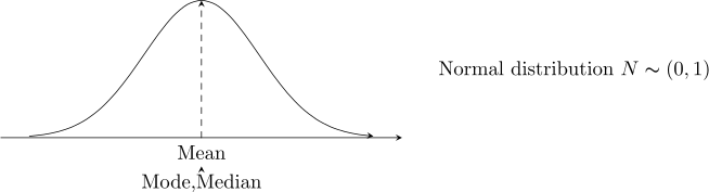
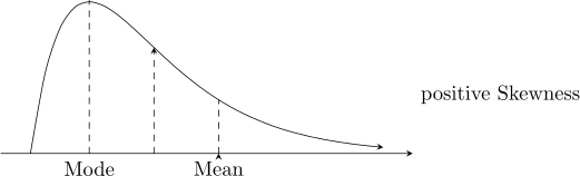
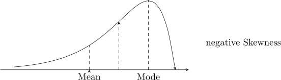
Coefficient of skewness measures the degree of lack of symmetry
\[SK=\frac {\text {Mean}\hspace {0.2cm}-\hspace {0.2cm}\text {Mode}}{\sigma }\]
\[SK=\frac {3(\text {Mean}\hspace {0.2cm}-\hspace {0.2cm} \text {Median})}{\sigma }\]
\[SK=\frac {Q_1+Q_3-2\text {Median}}{Q_3-Q_1}\]
\[SK=\frac {\sqrt {\beta _1}(\beta _2+3)}{2(5\beta _2-6\beta _1-a)}\]
Interpretation
- 1.
- If \(SK=0\), then the distribution symmetric.
- 2.
- If \(SK>0\), then the distribution is positively skewed.
- 3.
- If \(SK<0\), then the distribution is negatively skewed.
KURTOSIS is a measure of the degree of peakedness.
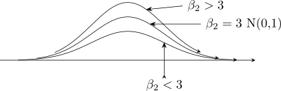
Coefficient of Kurtosis is calculated as: \[CK=\frac {\text {Semi Interquartile Range}}{P_{90}-P_{10}}\] The distribution is normal if \(CK=0.263\), otherwise the distribution is not normal.
Example 1.48. Given the data below
| C-I | \(0-2\) | \(2-4\) | \(4-6\) | \(6-8\) | \(8-10\) | \(10-12\) | \(12-14\) |
| \(f\) | 1 | 3 | 5 | 2 | 6 | 2 | 1 |
| \(X\) | 1 | 3 | 5 | 7 | 9 | 11 | 13 |
Using \(a=7\) as an arbitrary value.
- 1.
- Find the first four central moments.
- 2.
- Calculate \(\beta _1\) and \(\beta _2\).
- 3.
- Calculate the coefficient of skewness.
- 4.
- Calculate the coefficient of kurtosis, and comment.
Solution. The classes all have width \(h=2\), so instead of working with \(X\) directly we work with the coded value \[d=\frac {X-a}{h}=\frac {X-7}{2}\] This is not a trick to save arithmetic only. Shifting by \(a\) changes no central moment at all, and dividing by \(h\) scales the \(r\)th one by a known factor, so we can undo both at the end.
| C-I | \(f\) | \(X\) | \(d\) | \(fd\) | \(fd^2\) | \(fd^3\) | \(fd^4\) |
| \(0-2\) | 1 | 1 | \(-3\) | \(-3\) | 9 | \(-27\) | 81 |
| \(2-4\) | 3 | 3 | \(-2\) | \(-6\) | 12 | \(-24\) | 48 |
| \(4-6\) | 5 | 5 | \(-1\) | \(-5\) | 5 | \(-5\) | 5 |
| \(6-8\) | 2 | 7 | 0 | 0 | 0 | 0 | 0 |
| \(8-10\) | 6 | 9 | 1 | 6 | 6 | 6 | 6 |
| \(10-12\) | 2 | 11 | 2 | 4 | 8 | 16 | 32 |
| \(12-14\) | 1 | 13 | 3 | 3 | 9 | 27 | 81 |
| Total | 20 | \(-1\) | 49 | \(-7\) | 253 | ||
(1) The first four central moments.
The moments about \(a\), in coded units, are the column totals divided by \(n=20\): \begin {align*} m'_1 &=\frac {\sum fd}{n}=\frac {-1}{20}=-0.05 & m'_2 &=\frac {\sum fd^2}{n}=\frac {49}{20}=2.45\\ m'_3 &=\frac {\sum fd^3}{n}=\frac {-7}{20}=-0.35 & m'_4 &=\frac {\sum fd^4}{n}=\frac {253}{20}=12.65 \end {align*}
The mean follows at once, since \(\overline {X}=a+h\,m'_1\): \[\overline {X}=7+2(-0.05)=6.9\]
Now convert to moments about the mean with the formulas of the previous section: \begin {align*} \mu _2 &=m'_2-(m'_1)^2 = 2.45-(-0.05)^2=2.4475\\ \mu _3 &=m'_3-3m'_1m'_2+2(m'_1)^3 = -0.35-3(-0.05)(2.45)+2(-0.05)^3=0.01725\\ \mu _4 &=m'_4-4m'_1m'_3+6(m'_1)^2m'_2-3(m'_1)^4\\ &=12.65-4(-0.05)(-0.35)+6(-0.05)^2(2.45)-3(-0.05)^4=12.6167 \end {align*}
These are still in coded units. Multiplying the \(r\)th moment by \(h^r=2^r\) puts them back into the original units of \(X\): \begin {align*} \mu _2 &=2.4475\times 2^2 =9.79 & \mu _3 &=0.01725\times 2^3 =0.138\\ \mu _4 &=12.6167\times 2^4 =201.867 & \mu _1 &=0 \quad \text {always} \end {align*}
So the variance is \(9.79\) and the standard deviation \(\sqrt {9.79}=3.129\).
(2) \(\beta _1\) and \(\beta _2\). \begin {align*} \beta _1 &=\frac {\mu _3^{\,2}}{\mu _2^{\,3}}=\frac {(0.138)^2}{(9.79)^3}=\frac {0.019044}{938.31}=0.0000203\\ \beta _2 &=\frac {\mu _4}{\mu _2^{\,2}}=\frac {201.867}{(9.79)^2}=\frac {201.867}{95.844}=2.106 \end {align*}
Both are pure numbers with no units, which is the whole point of dividing by a power of \(\mu _2\). Had we forgotten to convert out of coded units, we would have got the same two answers, because \(\beta _1\) and \(\beta _2\) do not depend on \(h\) at all.
(3) Coefficient of skewness. \[\gamma _1=\sqrt {\beta _1}=\sqrt {0.0000203}=0.0045\] taking the sign of \(\mu _3\), which is positive.
(4) Coefficient of kurtosis. \[\gamma _2=\beta _2-3=2.106-3=-0.894\]
Comment.
\(\gamma _1=0.0045\) is as close to zero as makes no difference, so the distribution is symmetric for practical purposes.
There is a slight lean to the right, but a value that small should not be read as evidence of
anything.
\(\gamma _2=-0.894\) is negative, so the distribution is platykurtic: flatter in the middle and lighter in the tails than a normal curve. Look back at the frequencies to see why. They run \(1,3,5,2,6,2,1\) — there is no single tall peak, and the values are spread fairly evenly across the range instead of crowding round the centre. That is exactly the shape \(\beta _2<3\) describes.
Questions on this section
Stuck on something here? Ask below and it stays attached to this topic.