3.1 The \(P\)-value
Definition 3.1. The \(P\)-value is the probability of obtaining a result at least as extreme as the one observed, assuming the null hypothesis is true.
Every word of that matters, and the last clause most of all. The \(P\)-value is computed in a world where \(H_0\) holds. It answers “if nothing were going on, how often would I see something this striking?” – a small value means the data sit awkwardly with \(H_0\).
The decision rule. Reject \(H_0\) when \[P\text {-value} < \alpha .\] Always compare with \(\alpha \) itself, never with \(\alpha /2\). The halving belongs to the critical value in a two-tailed test, where each tail gets \(\alpha /2\). It is applied once, not twice:
- One-tailed test: \(P = P(Z > z_{\text {obs}})\), the single tail beyond the statistic.
- Two-tailed test: \(P = 2\times P(Z > |z_{\text {obs}}|)\) – double it, because a departure of that size in the opposite direction would have been just as surprising.
Doubling the tail and halving \(\alpha \) would penalise the same two-sidedness twice.
The two approaches always agree. The critical-value method asks whether the statistic is beyond the boundary; the \(P\)-value method asks how far beyond it is. The \(P\)-value carries more information – \(P = 0.049\) and \(P = 0.001\) both “reject at \(5\%\)” while saying very different things about the strength of the evidence.
3.1.1 What the \(P\)-value does not mean
These misreadings are common enough to be worth stating plainly.
- 1.
- It is not the probability that \(H_0\) is true. \(H_0\) is either true or it is not; it has no probability. The \(P\)-value is a probability about the data, computed assuming \(H_0\) – not a probability about the hypothesis.
- 2.
- It is not the probability that the result is due to chance.
- 3.
- \(1-P\) is not the probability that \(H_1\) is true. A \(P\)-value of \(0.03\) does not make \(H_1\) \(97\%\) likely.
- 4.
- A large \(P\)-value does not show \(H_0\) is true. It shows the data are consistent with \(H_0\). With a small sample, they would be consistent with much else besides.
- 5.
- Statistical significance is not practical importance. A large enough sample will return a small \(P\)-value for a difference far too slight to matter. Always ask how big the effect is, not merely whether it is significant.
- 6.
- \(\alpha =0.05\) is a convention, not a law of nature. There is nothing qualitatively different between \(P = 0.049\) and \(P = 0.051\), and reporting the actual \(P\)-value is more honest than reporting only “significant” or “not significant”.
3.1.2 Directed Hypothesis Test
One tailed test
\(H_0:\mu =a\hspace {1cm} H_0:\mu _1=\mu _2\)
\(H_1:\mu >a\hspace {1cm} H_1:\mu _1>\mu _2\)
\(H_1:\mu <a\hspace {1cm} H_1:\mu _1<\mu _2\)
Example 3.2. A machine fills bags of maize meal. When correctly set it delivers a mean of \(1000\) g per bag, and the filling weights are normally distributed with a standard deviation of \(5\) g which the machine’s design fixes and which does not drift. A quality inspector weighs a sample of \(n=9\) bags and finds a mean of \(\overline {X}=1003\) g.
Is there evidence, at the \(5\%\) level, that the machine is no longer correctly set?
Solution.
- 1.
-
- (a)
- Set up the hypothesis. “Correctly set” means the mean is neither too high nor too low, so the alternative is two-sided: \[H_0:\ \text {the machine is correctly set},\qquad H_1:\ \text {the machine is not correctly set}\] or, in symbols, \[H_0:\ \mu =1000\,\text {g}\qquad \text {against}\qquad H_1:\ \mu \neq 1000\,\text {g}.\]
- (b)
- Set up the level of significance \(\alpha =5\%\)
- (c)
- Test statistic. The standard deviation of \(5\) g is a property of the machine, so \(\sigma \) is known and the statistic is \(Z\) — not \(t\), despite \(n=9\) being small. What a small sample does require is that the population be normal, which is given. \begin {align*} Z &=\frac {\overline {X}-\mu }{\sigma /\sqrt {n}}=\frac {1003-1000}{5/\sqrt {9}}=\frac {3}{5/3}=1.80\\ Z_{0.025}&=1.96 \end {align*}
- (d)
- Critical region
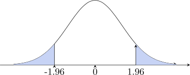
Figure 22: Two-tailed test at \(\alpha =5\%\): the rejection region is split between both tails. Interpretation: our statistic \(Z=1.80\) lies between \(-1.96\) and \(1.96\), in the acceptance region, so we fail to reject \(H_0\). At the \(5\%\) level there is no evidence that the machine is incorrectly set. The \(P\)-value is \(2P(Z>1.80)=0.072\), just above \(0.05\).
- 2.
- Now ask a different question: is the machine set too high? Naming a direction makes the test
one-tailed.
\[H_0:\ \text {the machine is correctly set},\qquad H_1:\ \text {the machine over-fills}\]
\[H_0:\ \mu =1000\,\text {g}\qquad \text {against}\qquad H_1:\ \mu >1000\,\text {g}\]
with \(\alpha =5\%\). The statistic is unchanged, \(Z=1.80\), but the critical value is not: all \(5\%\) now sits in one tail, so it is \(Z_{0.05}=1.645\)
rather than \(1.96\).
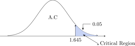
Figure 23: Acceptance and critical regions. \(Z=1.80\) exceeds \(Z_{0.05}=1.645\), so it falls in the critical region and we reject \(H_0\). The \(P\)-value is \(P(Z>1.80)=0.036\), below \(0.05\).
At the \(5\%\) level, then, the machine is over-filling.
Remark 3.3. The same data, the same statistic \(Z=1.80\), and two different answers — because the two questions are different. Asking ”is it correctly set?” leaves \(5\%\) to be split between two tails, so the bar is \(1.96\) and \(1.80\) does not clear it. Asking ”is it set too high?” puts the whole \(5\%\) in one tail, the bar drops to \(1.645\), and the same evidence now clears it.
Nothing is contradictory here, but the direction must be chosen before the data are seen. Running the two-tailed test, seeing it fail, and then switching to the one-tailed version to obtain a rejection is not a legitimate procedure — it doubles the true error rate.
Example 3.4. A clinic states that patients wait on average \(60\) minutes to be seen. A patients’ association suspects the true average is longer. It records the waiting times of a random sample of \(n=50\) patients and finds a mean of \(\overline {X}=64\) minutes with a standard deviation of \(S=6.3\) minutes.
Test, at the \(1\%\) level, whether the average waiting time exceeds the \(60\) minutes claimed.
Solution.
- 1.
- Set up the hypothesis. The association suspects the wait is longer, which names a direction, so the test is one-tailed: \[H_0:\ \text {the average wait is as claimed},\qquad H_1:\ \text {the average wait is longer}\] \[H_0:\ \mu =60\ \text {minutes}\qquad \text {against}\qquad H_1:\ \mu >60\ \text {minutes}.\]
- 2.
- Set up the level of significance at \(\alpha =1\%\).
- 3.
- Test statistic. Here \(\sigma \) is unknown and estimated by \(S\), but \(n=50>30\) is large, so \(Z\) serves: \begin {align*} Z &=\frac {\overline {X}-\mu }{S/\sqrt {n}}=\frac {64-60}{6.3/\sqrt {50}}=\frac {4}{0.891}=4.49 \end {align*}
(If \(S\) had been computed with divisor \(n\) rather than \(n-1\), the equivalent form is \(S/\sqrt {n-1}=6.3/7=0.9\), giving \(Z=4.44\). The two conventions differ trivially here and not at all in the conclusion.)
- 4.
- Critical region
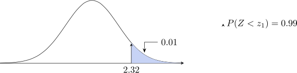
Figure 24: Locating the critical value from the tabulated probability. - 5.
- Conclusion. \(Z=4.49\) lies far beyond the critical value \(Z_{0.01}=2.326\), so we reject \(H_0\). There is very strong evidence, at the \(1\%\) level, that the average waiting time exceeds the \(60\) minutes the clinic states. The \(P\)-value is about \(0.0000036\) — if the true average really were \(60\) minutes, a sample mean this high would occur roughly once in \(280\,000\) samples.
Two things the test does not establish, worth stating because they are easy to slide into. It does not say the wait is much longer: the estimated excess is \(4\) minutes, and with \(n=50\) even a small excess is detectable. Significance measures the strength of the evidence, not the size of the effect. And it says nothing about why the wait is longer than claimed — these are observed times, not an experiment.
Questions on this section
Stuck on something here? Ask below and it stays attached to this topic.