5.2 Scatter diagram
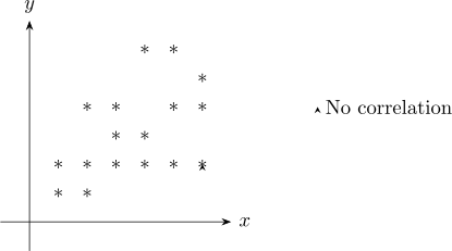
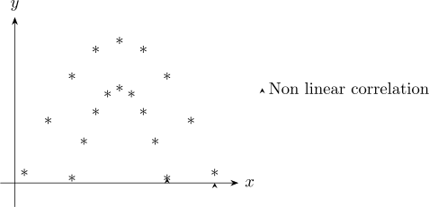
This involves plotting the variables on the \(X-Y\) plane and interpret the diagram, using standard diagrams
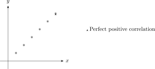
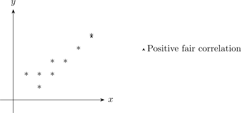
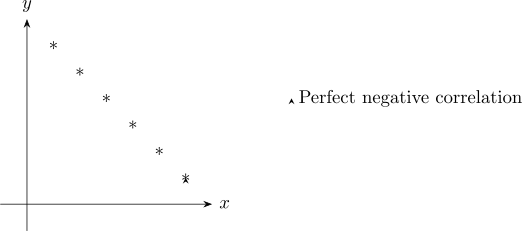
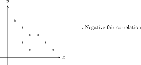
Example 5.1. The marks obtained by ten candidates in two papers are:
| Paper 1 | 42 | 84 | 50 | 42 | 33 | 50 | 69 | 81 | 80 | 35 |
| Paper 2 | 31 | 83 | 42 | 60 | 28 | 63 | 59 | 92 | 73 | 40 |
Draw a scatter diagram and interpret it.
Solution. Plotting Paper 1 horizontally against Paper 2 vertically gives points that rise from lower left to upper right in a fairly narrow band. Reading the diagram:
- (a).
- Direction. The pattern slopes upward, so the association is positive: candidates who scored well on Paper 1 tended to score well on Paper 2.
- (b).
- Form. The points fall roughly along a straight line rather than a curve, so a linear description is reasonable – which is what justifies computing a correlation coefficient at all.
- (c).
- Strength. The band is fairly tight but not perfect. Computing the coefficient confirms the reading: \(r=0.88\).
- (d).
- Outliers. No point sits far away from the pattern.
Since \(r^2=0.77\), about \(77\%\) of the variation in Paper 2 marks is accounted for by Paper 1 marks – unsurprising, since both are largely measuring the same candidates’ ability.
Remark 5.2. Always draw the diagram before computing \(r\). The coefficient measures linear association only, and it can be badly misleading on its own: data lying on a perfect curve can return an \(r\) near zero, and a single outlier can create a large \(r\) where the remaining points show no pattern whatever. The picture reveals both; the number hides them.
In order for you to talk about correlation between two variables, the two variables should be
related.
Questions on this section
Stuck on something here? Ask below and it stays attached to this topic.