3.2 Test for the Variance and Standard Deviation
When analysing numerical data sometimes you want to draw conclusion about the population variance
on s.d. For example if you are told that in a cereal filling process the population s.d. \(\sigma \) is equal to 15
grams. To see if the variability of the process has changed you need to test whether the s.d. has
changed from the previous specified level of 15 grams.
Assume that the data are normally distributed, you use the \(\chi ^2\) test for the variance \(\sigma \) s.d. to test whether
the population variance is equal to specified value.
Procedure
- 1.
- Set up the hypothesis.
- 2.
- Set \(\alpha \)
\(H_0: \sigma ^2 = S^2\)
\(H_1: \sigma ^2\neq S^2\) for two tailed test.
\(H_1:\sigma ^2>S^2\) for the upper one handed test.
\(H_1: \sigma ^2<S^2\) for the lower one handed test. - 3.
- Test statistic \[\chi ^2=(n-1)\frac {S^2}{\sigma ^2}\]
- 4.
- Critical Region
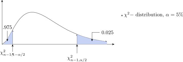
Figure 25: The chi-square distribution is not symmetric, so the two critical values must be looked up separately. The formula for the hypothesis can easily be converted to form an interval estimate for the variance \[\frac {(n-1)S^2}{\chi ^2_{\alpha /2,n-1}}\leq \sigma ^2\leq \frac {(n-1)S^2}{\chi ^2_{1-\alpha /2,n-1}}\]
Confidence interval for the ratio of variances \[\frac {S_1^2}{S^2_2}\,\cdot \,\frac {1}{F_{\frac {\alpha }{2},n_1-1,n_2-1}}\leq \frac {\sigma ^2_1}{\sigma _2^2}\leq \frac {S_1^2}{S_2^2}\,\cdot \, F_{\frac {\alpha }{2},n_2-1,n_1-1}\]
3.2.1 Chi-Square Tests
\(\chi ^2\) distribution
- \(\bullet \)
- It has only one parameter, called the degrees of freedom (df)
- \(\bullet \)
- The random variable \(\chi ^2\) assumes non negative values only.
- \(\bullet \)
- The shape of a Chi-square distribution curve is skewed to the right for small df and becomes symmetric for large df.
- \(\bullet \)
- The entire \(\chi ^2\)-distribution curve lies to the right of the vertical axis.
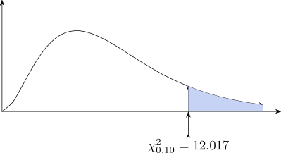
Example 3.5. Find the value of \(\chi ^2\) for 7 degrees of freedom and an area of 0.10 in the right tail
of the Chi square distribution curve.
Solution. From the table, locate 7 in the column for df and 0.10 in top row
Example 3.6. Find the value of \(\chi ^2\) for 12 degrees of freedom and an area of 0.5 in the left tail
of the Chi-square distribution curve.
Solution. Area in the right tail = \(1 - \) Area in the left \(= 1 - 0.05=0.95\)
Next, we locate 12 in the column for df and 0.950 in the top row \(\chi ^2_{.950,12}=5.226\)
Example 3.7. A dairy processing company claims that the variance of the amount of fat in
the whole milk processed by the company is no more than 0.25. You suspect this is wrong and
find that a random sample of 41 milk contains has a variance of 0.27. At \(\alpha =5\%\) is this enough evidence
to reject the company’s claims? Assume the population is normally distributed.
Solution.
- 1.
- Set up the hypothesis
\(H_0:\sigma ^2 \leq 0.25\)
\(H_1:\sigma ^2>0.25\)
- 2.
- Set \(\alpha =5\%\) level of significance.
- 3.
- Test Statistic
We have \(n=41,\hspace {0.4cm} \sigma ^2=0.25,\hspace {0.4cm} S^2=0.27,\hspace {0.4cm}\) df = 40 \begin {align*} \chi ^2 &=(n-1)\frac {S^2}{\sigma ^2}=\frac {(41-1)(0.27)^2}{(0.25)^2}\\\\ \implies \hspace {0.6cm} \chi ^2 &\approx 43.2\\ \end {align*} - 4.
- Critical Region
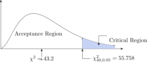
Figure 27: Test for a variance: the statistic \(\chi ^2=43.2\) against the critical value. Interpretation: Our statistic \(\chi ^2=43.2\) is less than the critical value, \(\chi ^2_{0.05}=55.758\). That is our statistic lies in the Acceptance region.
We accept \(H_0\) and reject \(H_1\), that is the company’s claims is true.
Example 3.8. A cereal process is set to a standard deviation of 15 grams. A sample of 25 packets has a standard deviation of \(17.7\) grams. Is there enough evidence that the process has changed?
Solution. “Changed” names no direction, so this is two-tailed. Testing \[H_0:\sigma =15 \qquad \text {against}\qquad H_1:\sigma \neq 15,\] the test statistic for a variance is \[\chi ^2=\frac {(n-1)s^2}{\sigma _0^2}=\frac {24(17.7)^2}{15^2} =\frac {24(313.29)}{225}=33.42,\] on \(n-1=24\) degrees of freedom.
Because the chi-square distribution is not symmetric, the two critical values must be looked up separately – there is no sign-flipping shortcut here. At \(\alpha =0.05\), \[\chi ^2_{0.975,\,24}=12.40 \qquad \text {and}\qquad \chi ^2_{0.025,\,24}=39.36.\] Our statistic \(33.42\) lies between them, so we fail to reject \(H_0\); the \(P\)-value is \(0.19\). There is not enough evidence that the process has changed.
Notice that the sample standard deviation, \(17.7\), is nearly \(18\%\) above the target, which looks substantial. With only 25 packets, however, a sample standard deviation that far out is not unusual – variances are estimated much less precisely than means, which is why the acceptance region here is so wide.
Questions on this section
Stuck on something here? Ask below and it stays attached to this topic.