1.10 Quartiles
Quartiles involves dividing the given ordered data into four equal points

1.10.1 Interquartile Range
This is a measure of dispersion which extends the ideal of the median. The median divides the data
into two equal parts. If we, now find the middle value of each half, we have for the lower half \(Q_1=\) lower
quartile and the upper half, we have the upper quartile \(=Q_3\). These divide the distribution into
quartiles.
\[\text {Interquartile Range}\hspace {0.3cm}=Q_3-Q_1\]
\[\text {Semi Interquartile Range}\hspace {0.3cm}=\frac {1}{2}(Q_3-Q_1)\]
We can see that the quartiles are \(\frac {1}{4}(n+1)^{\text {th}}\) value and \(\frac {3}{4}(n+1)^{\text {th}}\) values.
Example 1.40. Find the interquartile range of the data below.
| \(X\) | 1 | 2 | 3 | 4 | 5 | 6 | 7 | 8 | 9 | 10 |
| \(f\) | 2 | 8 | 9 | 5 | 4 | 3 | 4 | 1 | 1 | 1 |
Solution. Quartiles are found by position, so first accumulate the frequencies. Here \(n=38\).
| \(X\) | 1 | 2 | 3 | 4 | 5 | 6 | 7 | 8 | 9 | 10 |
| \(f\) | 2 | 8 | 9 | 5 | 4 | 3 | 4 | 1 | 1 | 1 |
| Cumulative \(f\) | 2 | 10 | 19 | 24 | 28 | 31 | 35 | 36 | 37 | 38 |
\(Q_1\) lies at position \(\tfrac {1}{4}(38)=9.5\), so it is the 10th ordered value. The cumulative frequency reaches 10 at \(X=2\), so \(Q_1=2\).
\(Q_3\) lies at position \(\tfrac {3}{4}(38)=28.5\), so it is the 29th value. The cumulative frequency passes 29 at \(X=6\), so \(Q_3=6\).
\[\text {IQR}=Q_3-Q_1=6-2=4.\]
The interquartile range covers the middle half of the data and, unlike the range, ignores both tails entirely. That is its purpose: the single observation at \(X=10\) stretches the range to 9, but moves the IQR not at all.
1.10.2 Interquartile Range for grouped data
For the data grouped into class interval we can estimate the quartiles from cumulative frequency curve
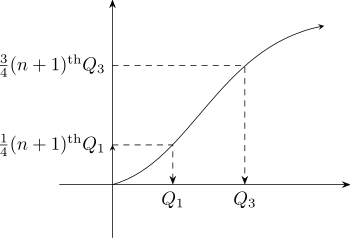
If \(\sum f=10\)
\(Q_1\) is the \(\frac {11}{4}^{\text {th}}\) observation \(\frac {11}{4}=2.75\implies Q_1\) lies between the 2\(^{\text {nd}}\) value and the \(3^{\text {nd}}\) value.
\(Q_3\) is the \(\frac {3}{4}\times 11^{\text {th}}\) observation \(\frac {3}{4}\times 11=\frac {33}{4}=8.25\implies Q_3\) lies between \(8^{\text {th}}\) value and \(9^{\text {th}}\) value.
Questions on this section
Stuck on something here? Ask below and it stays attached to this topic.