3 Statistical Hypothesis Testing
Deals with proving whether the given statement is true or false.
\(H_0:\) This is a positive statement which needs to be proved right or wrong (Null hypothesis).
For instance:
\(H_0:\) children in Zambia watch TV for 3 hours per week.
\(H_0: \mu =3\)
\(H_0:\) There is no difference in performance between boys and girls.
\(H_0: \mu _1=\mu _2\).
\(H_1:\) Is called alternative hypothesis. [Negative Statement]
Against the two null hypotheses above, these would be:
\(H_1 : \mu \neq 3\)
\(H_1: \mu _1 \neq \mu _2\)
The Four Steps of Hypothesis Testing
- 1.
- Set up the hypothesis
\(H_0:\) Null hypothesis which is positive statement to be proved.
\(H_1:\) Alternative hypothesis - 2.
- Set up the level of significance \(\alpha =\hspace {0.3cm}\text {level of significance}\)
- 3.
- Test statistic
We calculate the statistic and possible statistic are- (a)
- \(\displaystyle {Z=\frac {\overline {X}-\mu }{\text {S.e}}=\frac {\overline {X}-\mu }{\sigma /\sqrt {n}}\hspace {1cm}\text {or}\hspace {1cm}\frac {\overline {X}-\mu }{S/\sqrt {n-1}}\hspace {1cm}\text {or}\hspace {1cm}\frac {\overline {X}-\mu }{\hat {S}/\sqrt {n}}}\)
- (b)
- \(\displaystyle {Z=\frac {\overline {X}-\mu }{\sigma /\sqrt {n}}\hspace {0.6cm}\text {for}\hspace {0.3cm}n= \text {large},\hspace {0.3cm} \sigma = \text {known}}\)
\(\displaystyle {t_{n-1}=\frac {\overline {X}-\mu }{\sigma /\sqrt {n}}\hspace {0.6cm}\text {for}\hspace {0.3cm} n<30,\hspace {0.3cm} \sigma =\text {unknown}}\)
\(\displaystyle {t_{n-1}=\frac {\overline {X}-\mu }{\hat {S}/\sqrt {n}}\hspace {1cm}\text {and}\hspace {1cm}t_{n-1}=\frac {\overline {X}-\mu }{\sigma /\sqrt {n}}}\)
- (c)
- Difference between two means.
When \(n\) is large and \(\sigma _1\) and \(\sigma _2\) are known. \[Z=\frac {(\overline {X}_1-\overline {X}_2)-(\mu _1-\mu _2)}{\sqrt {\frac {\sigma ^2_1}{n_1}+\frac {\sigma ^2_2}{n_2}}},\hspace {2cm} Z=\frac {\overline {X}_1-\overline {X}_2}{\sqrt {\frac {\sigma ^2_1}{n_1}+\frac {\sigma ^2_2}{n_2}}}\]
\[t_{n_1+n_2-2}=\frac {\overline {X}_1-\overline {X}_2}{\sqrt {\frac {n_1S^2_1+n_2S^2_2}{n_1+n_2-2}\Bigg (\frac {1}{n_1}+\frac {1}{n_2}\Bigg )}}\hspace {0.6cm}n<30,\hspace {0.4cm}\sigma = \text {unknown}\]
Paired Test: \(\hspace {0.5cm} \displaystyle {t_{n-1}=\frac {\mu -\overline {d}}{\frac {\text {SD}}{\sqrt {n-1}}}}\)
Significance of a proportion: \(\hspace {0.5cm} \displaystyle {Z=\frac {\hat {P}-P}{\sqrt {\frac {P(1-P)}{n}}}}\) for large sample size.
- 4.
- Critical Region
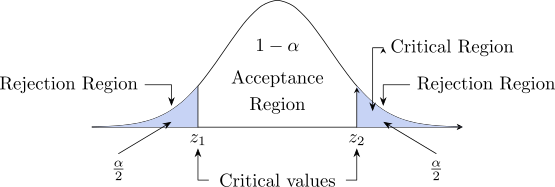
Figure 20: Acceptance and critical regions for a two-tailed test.
\(Z_{\alpha /2}\) undirected hypothesis tests, two tailed test \(\alpha =5\%\).
Interpretation: if the statistic \(Z\) falls in the critical region we reject \(H_0\) in favour of \(H_1\). If it does not, we fail to reject \(H_0\).
Say it that way, and not “\(H_1\) is true” or “\(H_0\) is true”. A test never establishes either hypothesis. Rejecting \(H_0\)
says the data would be unusual if \(H_0\) held, which is evidence against it – not proof of \(H_1\). Failing to reject
says only that the data are consistent with \(H_0\); they may be consistent with a great many other
values too, particularly when the sample is small. Absence of evidence is not evidence of
absence.
We can use the P-value for interpretation given statistic \(\alpha =0.025\) , \(Z=2.13\)
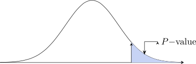
\begin {align*} P(Z>2.13) &=1-P(Z\leq 2.13)=1-0.9834\\ &=0.016 \end {align*}
Because the test is two-tailed, a result this far from the centre is equally surprising in either direction, so the \(P\)-value is both tails together: \[P\text {-value} = 2\times P(Z>2.13) = 2\times 0.0166 = 0.033.\] Since \(0.033 < \alpha = 0.05\), we reject \(H_0\).
3.1.1 What the \(P\)-value does not mean
3.1.2 Directed Hypothesis Test
3.2 Test for the Variance and Standard Deviation
3.2.1 Chi-Square Tests
3.3 Type I and Type II Errors
3.4 Test of Independence and Goodness of Fit Test
3.5 Tests Comparing Two Populations
3.5.1 Two means, \(\sigma _1\) and \(\sigma _2\) known
3.5.2 Two means, \(\sigma _1=\sigma _2\) unknown — the pooled \(t\)-test
3.5.3 Paired samples — the paired \(t\)-test
3.5.4 Two proportions
3.5.5 Two variances — the \(F\)-test
3.5.6 Choosing between them
3.6 Practice Problems
Questions on this section
Stuck on something here? Ask below and it stays attached to this topic.