1.2 Continuous Data
Continuous data can take any value within a range, with no gaps: between any two values, however close, another is possible. Such data arise from measuring rather than counting.
The distinction is about what the quantity can be, not how it is written down. Height recorded to
the nearest centimetre is still continuous – the rounding is a limit of the ruler, not of the
person.
Examples of continuous variables include:
- 1.
- Age
- 2.
- Time
- 3.
- Weight
- 4.
- Height
To present continuous data we also use
- 1.
- Line Plots
- 2.
- Histogram
- 3.
- Frequency polygon
- 4.
- Ogive curve (Cumulative frequency curve)
- 5.
- Steam and Leaf plots
- 6.
- Two-Way tables
- 7.
- Box plots
- 8.
- Scatter plots
- 9.
- Time-Series plots
Line Plots
- \(\bullet \)
- Analysis begins by trying to get a good “picture” of the data.
- \(\bullet \)
- A line plot is simply a bar plot (bar graph) where the categories on which we collect data
are integers \((0,1,2,3,\ldots ,\cdots )\).
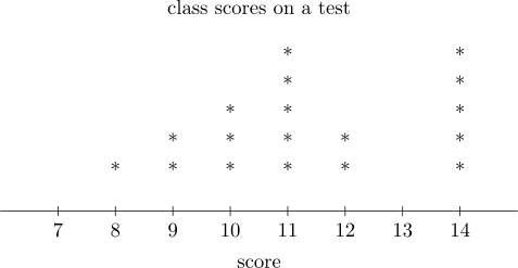
The method of construction:
- Step 1: Find the smallest and largest values in the data set.
- Step 2: Draw a real number line that encompasses these values.
- Step 3: Place a mark on the number line corresponding to each data point.
Solution.
Frequency, Relative Frequency, and Cumulative Frequency
- \(\bullet \)
- A frequency is the number of times a given datum occurs in a data set.
- \(\bullet \)
- A relative frequency is the fraction of times an answer occurs. To find the relative
frequencies, divide each frequency by the total number in the sample.
Relative frequencies can be written as fractions, percents, or decimals.Data Value Frequency Relative Frequency 2 3 3/20 or 0.15 3 5 5/20 or 0.25 4 3 3/20 or 0.15 5 6 6/20 or 0.30 6 2 2/20 or 0.10 7 1 1/20 or 0.05 - \(\bullet \)
- The sum of the relative frequency column is 20/20, or 1.
- \(\bullet \)
- Cumulative relative frequency is the accumulation of the previous relative frequencies.
Cumulative Relative Data Value Frequency Relative Frequency Frequency 2 3 3/20 or 0.15 0.15 3 5 5/20 or 0.25 0.15 + 0.25=0.40 4 3 3/20 or 0.15 0.40 + 0.15=0.55 5 6 6/20 or 0.30 0.55 + 0.30=0.85 6 2 2/20 or 0.10 0.85 + 0.10=0.95 7 1 1/20 or 0.05 0.95 + 0.05=1.00
Note 1.8. Because of rounding, the relative frequency column may not always sum to one and
the last entry in the cumulative relative frequency column may not be one. However, they each
should be close to one.
We can arrange data into groups or take them as individual values.
If we consider 5 values, say 3, 5, 0, 2, 6.
In grouping data, we can either take individual values or arrange then in intervals called class
interval.
| Value | Tally Marks | \(f\) |
| 0 |  | 5 |
| 1 |  | 2 |
| 2 |  | 1 |
| 3 |  | 3 |
To determine class interval, find the range and divide by 10
| Class | Tally | \(f\) | True Class |
| Interval | Marks | Limits | |
| \(1-5\) |  | 1 | \(0.5-5.5\) |
| \(6-10\) |  | 2 | \(5.5-10.5\) |
| \(11-15\) |  | 3 | \(10.5-15.5\) |
| \(16-20\) |  | 1 | \(15.5-20.5\) |
| \(21-25\) |  | 2 | \(20.5-25.5\) |
| \(26-30\) |  | 1 | \(25.5-30.5\) |
1.2.1 Choice Of Class Interval
1.2.2 How many classes? The \(2^k\) rule and Sturges’ formula
The paragraph above says a class interval should be neither too wide nor too narrow, which is true and not much help. With a handful of observations the choice can be made by eye. Once \(N\) runs into the hundreds it cannot, and guessing wastes time and produces tables that disagree with each other for no reason.
Two rules settle the question. Both fix the number of classes \(k\) first, and let the class width follow.
The \(2^k\) rule. Choose the smallest whole number \(k\) for which \[2^k\geq N.\] The reasoning is a counting one: with \(k\) classes there are \(2^k\) possible patterns of ”in or out”, and we want at least as many as there are observations, so that the classes are capable of separating them.
Sturges’ formula. Take \[k=1+3.322\log _{10}N.\]
The two are the same rule. That \(3.322\) is not arbitrary: \[\frac {1}{\log _{10}2}=3.3219\ldots \] so \(3.322\log _{10}N=\log _2 N\), and Sturges’ formula is simply \[k=1+\log _2 N,\] while the \(2^k\) rule gives \(k=\lceil \log _2 N\rceil \). Sturges therefore returns about one class more than the \(2^k\) rule — never a wildly different answer, and either is defensible.
Then the width. With \(k\) decided, \[i=\frac {\text {range}}{k}=\frac {\text {largest}-\text {smallest}}{k}\] rounded up to a convenient number. Round up, not down: rounding down can leave the largest observation outside the last class. And choose something a reader can hold in their head — \(5\), \(10\), \(2.5\) — rather than the raw \(2.333\) the division happens to give.
| \(N\) | 20 | 30 | 50 | 100 | 200 | 500 | 1000 | 5000 |
| \(2^k\geq N\) | 5 | 5 | 6 | 7 | 8 | 9 | 10 | 13 |
| Sturges | 5 | 6 | 7 | 8 | 9 | 10 | 11 | 13 |
The slow growth in that table is the useful part. Going from \(50\) observations to \(5000\) — a hundredfold increase — takes the number of classes only from \(6\) to \(13\). A reader who expects a thousand observations to need dozens of classes is expecting the wrong thing.
Example 1.9. Fifty measurements of antibody concentration range from \(5.2\) to \(19.2\) g/l. How many classes should the frequency distribution have, and how wide?
Solution. By the \(2^k\) rule. \(2^5=32<50\) and \(2^6=64\geq 50\), so \(k=6\).
By Sturges’ formula. \[k=1+3.322\log _{10}50=1+3.322(1.699)=1+5.644=6.64\approx 7.\]
The two differ by one, as they generally do. Taking \(k=7\): \[i=\frac {19.2-5.2}{7}=\frac {14.0}{7}=2.0,\] so seven classes of width \(2\), starting at \(5.2\): \(5.2-7.2\), \(7.2-9.2\), and so on up to \(17.2-19.2\).
Notice that the division came out exactly, so the largest observation, \(19.2\), sits precisely on the upper boundary of the last class. The last class must therefore be closed at both ends — written \([17.2,\,19.2]\) while the others are \([a,\,b)\) — or \(19.2\) belongs to no class at all. The alternative is to round the width up slightly anyway, to \(2.5\), and accept a little spare room at the top.
Taking \(k=6\) instead gives \(i=14.0/6=2.33\), rounded up to \(2.5\), and the question does not arise.
Either is a reasonable table. What the rules have done is narrow an unlimited choice to two sensible candidates, in a few seconds, with a defensible reason.
Example 1.10. A survey records the monthly income of \(850\) households, the lowest being K\(400\) and the highest K\(9\,800\). Construct a suitable class structure.
Solution. Number of classes. \(2^9=512<850\) and \(2^{10}=1024\geq 850\), so the \(2^k\) rule gives \(k=10\). Sturges gives \[k=1+3.322\log _{10}850=1+3.322(2.929)=1+9.73=10.7\approx 11.\]
Width. The range is \(9800-400=9400\), so with \(k=10\) \[i=\frac {9400}{10}=940.\] Nobody wants classes of width \(940\). Round up to \(1000\), which is both convenient and slightly generous: \[400-1400,\quad 1400-2400,\quad \ldots ,\quad 9400-10400.\] That is ten classes covering \(400\) to \(10\,400\), comfortably containing the largest value.
Rounding the width up is what makes the coverage work. Had \(900\) been chosen instead, ten classes would reach only \(400+9000=9400\) and the household earning K\(9\,800\) would have nowhere to go.
Remark 1.11. Both rules are starting points, not verdicts. Sturges’ formula is derived by matching a histogram to the binomial coefficients of a normal distribution, so it assumes the data are roughly normal and moderate in number. For very large samples, or for strongly skewed data, it is known to give too few classes and so to smooth away detail that is really there. If the resulting histogram looks suspiciously featureless, try more classes and see whether structure appears. The rule saves you from an arbitrary choice; it does not excuse you from looking at the result.
It is important that the class interval in chosen so that the graph gives a clear representation of the
Data. Choice of too large a class interval will lead to loss of details on the other hand too small a class
interval would destroy the originality of the Data. A Convenient rule of thumb is to choose a class
interval so that the Average frequency is about 5.
i.e. Number of classes = \(\frac {1}{5}\times \) Total frequency.
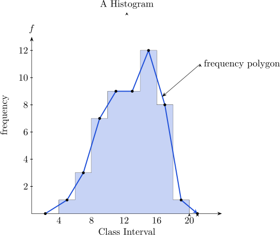
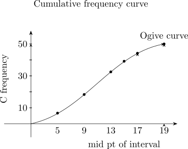
| Class | \(f\) | Cumulative | Middle Point |
| Interval | frequency | of the interval | |
| \(4.0-6\) | 1 | 1 | 5 |
| \(6.0-8\) | 3 | 4 | 7 |
| \(8.0-10\) | 7 | 11 | 9 |
| \(10.0-12\) | 9 | 20 | 11 |
| \(12.0-14\) | 9 | 29 | 13 |
| \(14.0-16\) | 12 | 41 | 15 |
| \(16.0-18\) | 8 | 49 | 17 |
| \(18.0-20\) | 1 | 50 | 19 |
Construct a Histogram using the given table:
Questions on this section
Stuck on something here? Ask below and it stays attached to this topic.