5.6 Practice Problems
Problem 5.1. Pupils transferring from primary to secondary education are given two verbal reasoning tests. The scores of twelve pupils, quoted relative to the mean score for each test, are:
| Pupil | A | B | C | D | E | F | G | H | I | J | K | L |
| Test 1 | \(-15\) | \(-14\) | \(-10\) | \(-5\) | \(-4\) | \(-1\) | 2 | 5 | 10 | 13 | 17 | 20 |
| Test 2 | \(-10\) | \(-7\) | \(-4\) | \(-6\) | \(-1\) | 6 | \(-2\) | 5 | 9 | 0 | 10 | 12 |
Show that the product-moment correlation coefficient of the test scores is approximately \(0.871\).
Show solution
Solution. Use the computational form, which avoids working out every deviation: \[r=\frac {n\sum XY-\sum X\sum Y} {\sqrt {n\sum X^2-\left (\sum X\right )^2}\ \sqrt {n\sum Y^2-\left (\sum Y\right )^2}}.\] From the table, with \(n=12\): \[\sum X=18,\quad \sum Y=12,\quad \sum XY=837,\quad \sum X^2=1550,\quad \sum Y^2=592.\] Then \[n\sum XY-\sum X\sum Y = 12(837)-(18)(12)=10044-216=9828,\] \[n\sum X^2-\left (\sum X\right )^2=12(1550)-324=18276,\] \[n\sum Y^2-\left (\sum Y\right )^2=12(592)-144=6960,\] so \[r=\frac {9828}{\sqrt {18276}\ \sqrt {6960}}=\frac {9828}{135.19\times 83.43}=0.871,\] as required.
A word on why the scores being “quoted relative to the mean” does not matter. Correlation is unaffected by adding a constant to either variable, so subtracting each test’s mean beforehand leaves \(r\) exactly as it was. It only makes the arithmetic pleasanter.
An \(r\) of \(0.871\) is a strong positive association: pupils who did well on one test tended to do well on the other, which is what one would hope of two tests intended to measure the same thing.
Problem 5.2. In an experiment the values of two variables \(X\) and \(Y\) are measured. Ten experiments gave \[(6,13),\ (12,2),\ (9,12),\ (5,15),\ (2,17),\ (12,5),\ (8,10),\ (3,13),\ (11,12),\ (7,11).\]
- (a).
- Find the equation of the regression line of \(Y\) on \(X\).
- (b).
- Find \(r\) and \(R^2\), and say what they mean here.
- (c).
- Construct the ANOVA table and test whether the slope differs from zero.
Show solution
Solution. (a). With \(n=10\), \[\sum X=75,\quad \sum Y=110,\quad \sum XY=707,\quad \sum X^2=677.\] \[\hat {b}=\frac {n\sum XY-\sum X\sum Y}{n\sum X^2-\left (\sum X\right )^2} =\frac {10(707)-75(110)}{10(677)-75^2}=\frac {7070-8250}{6770-5625} =\frac {-1180}{1145}=-1.031.\] \[\hat {a}=\overline {Y}-\hat {b}\,\overline {X}=11-(-1.031)(7.5)=18.729.\] So the regression line is \[Y=18.729-1.031X.\] The negative slope says \(Y\) falls by about \(1.03\) units for each unit increase in \(X\). As a check, the line passes through \((\overline {X},\overline {Y})=(7.5,11)\), as it must.
(b). \(r=-0.822\) and \(R^2=0.676\).
The sign of \(r\) matches the sign of the slope, as it always does. \(R^2=0.676\) says the line accounts for about \(68\%\) of the variation in \(Y\); the remaining \(32\%\) is scatter about the line that \(X\) does not explain.
(c). The fitted values give \[SS_T=180.0,\qquad SS_R=121.61,\qquad SS_E=58.39,\] and \(SS_R/SS_T=0.676=R^2\), which is a useful arithmetic check.
| Source | \(SS\) | df | \(MS\) | \(F\) |
| Regression | \(121.61\) | \(1\) | \(121.61\) | \(16.66\) |
| Error | \(58.39\) | \(8\) | \(7.30\) | |
| Total | \(180.00\) | \(9\) |
Testing \(H_0:\beta =0\), the critical value is \(F_{1,8,\,0.05}=5.32\) and \(16.66\) is well beyond it. The \(P\)-value is \(0.0035\), so we reject \(H_0\): there is strong evidence of a linear relationship.
The equivalent \(t\)-test gives the same verdict. With \(s=\sqrt {MS_E}=2.70\) and \(\sum (X-\overline {X})^2=114.5\), \[SE(\hat {b})=\frac {2.70}{\sqrt {114.5}}=0.2525, \qquad t=\frac {-1.031}{0.2525}=-4.08\] on \(8\) degrees of freedom, against a critical \(2.306\) – and the same \(P\)-value of \(0.0035\). Note that \[t^2=(-4.08)^2=16.66=F,\] exactly as it must be: in simple linear regression the two tests are one test written two ways.
A \(95\%\) confidence interval for the slope is \[-1.031\pm 2.306(0.2525)=-1.031\pm 0.582=(-1.613,\ -0.449).\] It excludes zero, which is the same conclusion again – but it also says how large the effect plausibly is, which neither test does on its own.
Problem 5.3. Flowers were grown on standard plots inside and outside glasshouses. For each plot the amount of a vital but toxic chemical was measured, together with the average number of blooms. Calculate the product-moment correlation coefficient for each set.
| Chemical \(X\) (mg) | 3 | 4 | 6 | 7 | 8 | 10 | 12 | 15 | 16 |
| Blooms \(Y\) | 3.2 | 2.9 | 3.7 | 2.2 | 1.8 | 2.3 | 1.7 | 0.8 | 0.3 |
| Chemical \(X\) (mg) | 3 | 5 | 6 | 10 | 11 | 12 | 14 | 15 |
| Blooms \(Y\) | 4.0 | 4.2 | 3.6 | 2.3 | 2.5 | 1.9 | 1.3 | 1.1 |
Show solution
Solution. Both use \[r=\frac {S_{XY}}{\sqrt {S_{XX}S_{YY}}},\qquad S_{XY}=\sum XY-\frac {\sum X\sum Y}{n},\quad S_{XX}=\sum X^2-\frac {(\sum X)^2}{n}.\]
First set (\(n=9\)): \(\sum X=81\), \(\sum Y=18.9\), giving \[S_{XX}=170.0,\qquad S_{YY}=9.64,\qquad S_{XY}=-36.7\] \[r=\frac {-36.7}{\sqrt {170.0\times 9.64}}=\frac {-36.7}{40.48}=-0.907.\]
Second set (\(n=8\)): \(\sum X=76\), \(\sum Y=20.9\), giving \[S_{XX}=134.0,\qquad S_{YY}=10.05,\qquad S_{XY}=-35.95\] \[r=\frac {-35.95}{\sqrt {134.0\times 10.05}}=\frac {-35.95}{36.70}=-0.980.\]
Both are strong negative correlations: more chemical, fewer blooms. The second set is the tighter of the two, \(-0.980\) against \(-0.907\).
Two cautions. The chemical is described as vital as well as toxic, so the true relationship is unlikely to be a straight line over the whole range — too little would harm the plants as well. These data only cover the descending part of that curve. And correlation this strong still does not establish that the chemical causes the reduction; the plots inside and outside glasshouses may differ in other ways too.
Problem 5.4. A flower competition is to be judged on the opinions of judges X and Y:
| Competitor | A | B | C | D | E | F | G | H | I | J |
| Judge X | 48 | 50 | 55 | 51 | 51 | 47 | 48 | 46 | 52 | 50 |
| Judge Y | 18 | 19 | 29 | 22 | 26 | 14 | 22 | 11 | 24 | 17 |
- (a).
- Carry out a rank test to determine whether the two judges’ opinions are consistent.
- (b).
- Determine an order of merit for the competition.
Show solution
Solution. A rank test is the right tool here, and not merely an alternative to the product-moment coefficient. The two judges are using quite different parts of their scales — X’s marks run from \(46\) to \(55\), Y’s from \(11\) to \(29\) — so what matters is whether they put the competitors in the same order, not whether their numbers agree.
(a) Rank each judge’s marks, sharing ranks where there are ties:
| Competitor | A | B | C | D | E | F | G | H | I | J |
| Rank X | 3.5 | 5.5 | 10 | 7.5 | 7.5 | 2 | 3.5 | 1 | 9 | 5.5 |
| Rank Y | 4 | 5 | 10 | 6.5 | 9 | 2 | 6.5 | 1 | 8 | 3 |
| \(d\) | \(-0.5\) | 0.5 | 0 | 1.0 | \(-1.5\) | 0 | \(-3.0\) | 0 | 1.0 | 2.5 |
| \(d^2\) | 0.25 | 0.25 | 0 | 1.0 | 2.25 | 0 | 9.0 | 0 | 1.0 | 6.25 |
With \(\sum d^2=20\) and \(n=10\), \[r_s=1-\frac {6\sum d^2}{n(n^2-1)}=1-\frac {6(20)}{10(99)}=1-0.121=0.879.\] The critical value for \(n=10\) at the \(5\%\) level (two-tailed) is \(0.648\). Since \(0.879>0.648\), the judges’ opinions are consistent.
(b) Since the judges broadly agree, the sensible order of merit adds their ranks: C (\(10+10=20\)) first, then I (\(9+8=17\)), E (\(7.5+9=16.5\)), D (\(7.5+6.5=14\)), B (\(5.5+5=10.5\)), G (\(3.5+6.5=10\)), J (\(5.5+3=8.5\)), A (\(3.5+4=7.5\)), F (\(2+2=4\)), H (\(1+1=2\)).
Adding the raw marks would be wrong: Judge X’s range is only \(9\) marks wide while Judge Y’s is \(18\), so Y’s opinion would silently count for twice as much.
Problem 5.5. The table gives Mosi consumption in Lusaka in millions of litres.
| Year | 2000 | 2001 | 2002 | 2003 | 2004 | 2005 | 2006 | 2007 | 2008 | 2009 |
| Consumption | 3.5 | 37.1 | 35.5 | 37.5 | 41.5 | 46.4 | 44.8 | 45.8 | 53.9 | 62.0 |
- (a).
- Draw a scatter diagram.
- (b).
- Determine the least squares regression line of \(Y\) on \(X\).
- (c).
- Use it to estimate consumption for 2010.
- (d).
- Comment on the appropriateness of a linear model, given that actual 2010 consumption was \(78.3\) million litres.
Show solution
Solution. Before anything else. The \(2000\) figure of \(3.5\) sits among values of \(35\) to \(62\) and is followed by \(37.1\). It is almost certainly \(33.5\) with a digit dropped. The working below uses the data as given, and then shows what difference the anomaly makes — altering someone’s data without saying so is not an option.
(a), (b) Code the years as \(x=\text {year}-2000\), so \(x=0,1,\ldots ,9\). Then \(n=10\), \(\sum x=45\), \(\sum Y=408.0\), and \[S_{XX}=82.5,\qquad S_{XY}=361.2\] \[\widehat {b}=\frac {S_{XY}}{S_{XX}}=\frac {361.2}{82.5}=4.378,\qquad \widehat {a}=\overline {Y}-\widehat {b}\,\overline {x}=40.8-4.378(4.5)=21.10\] \[\implies \quad \widehat {Y}=21.10+4.378x.\]
(c) For \(2010\), \(x=10\): \[\widehat {Y}=21.10+4.378(10)=64.9\ \text {million litres}.\]
(d) The actual figure was \(78.3\), so the model is short by \(13.4\) million litres — about \(17\%\). Three things are going on.
First, the prediction is an extrapolation: \(x=10\) lies outside the range of the data, where a fitted line carries no guarantee at all.
Second, the anomalous first value drags the line down. Reading it as \(33.5\) instead gives \(\widehat {Y}=31.46+2.742x\), a \(2010\) prediction of \(58.9\) — further from the truth, but with \(r\) improving from \(0.860\) to \(0.935\). The single bad point was flattering the fit’s slope while spoiling its correlation.
Third, and most importantly, the residuals are not random: consumption is rising faster than linearly towards the end of the series, and \(2010\) continues that. A straight line is the wrong shape. A model allowing for growth — a quadratic, or a line fitted to \(\log Y\) — would suit these data better.
Problem 5.6. The table shows the mass of an animal at weekly intervals.
| Age (weeks) | 11 | 12 | 13 | 14 | 15 | 16 |
| Mass (kg) | 357 | 382 | 404 | 423 | 404 | 451 |
State whether it is more appropriate to fit a regression line of age on mass or mass on age, and justify your choice. What value does your line give for the mass at \(17\) weeks?
Show solution
Solution. Which line. Mass on age. The two regression lines answer different questions and are not interchangeable. Least squares minimises the squared deviations in the dependent variable only, so the choice depends on which variable is which. Here age is fixed by the experimenter — the animal was weighed at chosen weekly intervals, and those ages carry no measurement error — while mass is the response that varies. Age is therefore the independent variable and mass the dependent one.
Fitting it. With \(n=6\), \(\overline {x}=13.5\) and \(\overline {y}=403.5\): \[S_{XX}=17.5,\qquad S_{XY}=277.5\] \[\widehat {b}=\frac {277.5}{17.5}=15.86,\qquad \widehat {a}=403.5-15.86(13.5)=189.43\] \[\implies \quad \widehat {\text {mass}}=189.43+15.86\,(\text {age}).\]
At \(17\) weeks, \[\widehat {y}=189.43+15.86(17)=459.0\ \text {kg}.\]
Two reservations worth recording. The reading at week \(15\), \(404\) kg, is lower than week \(14\)’s \(423\) and identical to week \(13\)’s — an animal losing weight then gaining \(47\) kg in a week is odd, and it may be a recording error. And \(17\) weeks is beyond the data, so the estimate assumes growth continues at the same steady rate, which for a growing animal it eventually will not.
Problem 5.7. In an investigation of the effect of duration of training (\(X\)) on performance time (\(Y\)), observations from \(26\) trainees gave \[\sum x=104,\qquad \sum (x-\overline {x})^2=56,\qquad \sum (x-\overline {x})(y-\overline {y})=-56, \qquad \sum (y-\overline {y})^2=62.\]
- (a).
- Give the linear relationship of \(y\) to \(x\) which best fits the observations.
- (b).
- Calculate the value predicted for \(y\) when \(x=12\).
- (c).
- Estimate \(\sigma ^2_{y/x}\).
- (d).
- Calculate \(95\%\) confidence limits for \(\beta \).
Show solution
Solution. The question as printed gives \(\sum (y-\overline {y})=62\). That sum is identically zero for any data whatever, since deviations about their own mean always cancel. The intended quantity is \(\sum (y-\overline {y})^2=62\), and that is what is used here.
(a) \(\overline {x}=\frac {104}{26}=4\), and \[\widehat {b}=\frac {S_{XY}}{S_{XX}}=\frac {-56}{56}=-1.\] The value of \(\overline {y}\) is not given, so the intercept cannot be found as a number. The line is still fully determined in deviation form: \[y-\overline {y}=-1(x-4)\qquad \text {that is}\qquad \widehat {y}=\overline {y}-x+4.\] Longer training reduces performance time by one unit per unit of training.
(b) At \(x=12\), \[\widehat {y}=\overline {y}-12+4=\overline {y}-8,\] so the predicted performance time is \(8\) units below the mean. Without \(\overline {y}\) that is as far as the arithmetic can go, and it is a complete answer to what was asked.
(c) The residual sum of squares is \[SSE=S_{YY}-\widehat {b}\,S_{XY}=62-(-1)(-56)=6\] \[\implies \quad \widehat {\sigma }^2_{y/x}=\frac {SSE}{n-2}=\frac {6}{24}=0.25.\]
(d) The standard error of the slope is \[\text {se}(\widehat {b})=\sqrt {\frac {\widehat {\sigma }^2_{y/x}}{S_{XX}}}=\sqrt {\frac {0.25}{56}}=0.0668\] and with \(t_{24,\,0.025}=2.064\), \[-1\pm 2.064(0.0668)=-1\pm 0.138\quad \implies \quad (-1.138,\ -0.862).\] The interval is comfortably clear of zero, so the effect of training is significant. The fit is very tight — of the total \(62\) in \(Y\), all but \(6\) is explained by \(x\), giving \(r=-0.950\).
Problem 5.8. A state official was investigating the relationship between salary (\(x\)) and the number of absences (\(y\)) for state employees. The variable \(y\) in the following table represents the average number of absences per year for employees at that salary.
| Salary in $ thousands (\(x\)) | 20.0 | 22.5 | 25.0 | 27.5 | 30.0 | 32.5 | 35.0 | 37.5 | 40.0 |
| Number of absences (\(y\)) | 2.3 | 2.0 | 2.0 | 1.8 | 2.2 | 1.5 | 1.2 | 1.3 | 0.6 |
- (a).
- Draw a scatter diagram. Does a linear relationship between \(x\) and \(y\) seem appropriate?
- (b).
- Estimate the simple linear regression line. Interpret the parameters in the model.
- (c).
- Estimate the average number of absences for employees earning $29,000.
- (d).
- At the \(5\%\) level of significance would you conclude that there is a linear relationship between \(x\) and \(y\)?
- (e).
- Construct a \(95\%\) confidence interval for the slope parameter \(\beta \).
- (f).
- Find the coefficient of determination and interpret the value.
- (g).
- Find the correlation coefficient.
Show solution
Solution. All seven parts run off the same five sums, so they are computed once at the start. With \(n=9\), \[\sum x=270,\quad \sum y=14.9,\quad \sum xy=420,\quad \sum x^2=8475,\quad \sum y^2=27.11,\] \[\overline {x}=30.0,\qquad \overline {y}=1.6556,\] \begin {align*} S_{xx}&=\sum x^2-\frac {(\sum x)^2}{n}=8475-\frac {72{,}900}{9}=8475-8100=375,\\ S_{yy}&=\sum y^2-\frac {(\sum y)^2}{n}=27.11-\frac {222.01}{9}=27.11-24.6678=2.4422,\\ S_{xy}&=\sum xy-\frac {(\sum x)(\sum y)}{n}=420-\frac {(270)(14.9)}{9}=420-447=-27. \end {align*}
(a). The scatter diagram.
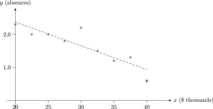
The points fall steadily from left to right and stay close to a straight line, so a linear relationship is appropriate. The trend is negative: employees on higher salaries are absent less often. Only the point at \(x=30\) (\(y=2.2\)) sits noticeably above the pattern.
(b). The regression line. \[b=\frac {S_{xy}}{S_{xx}}=\frac {-27}{375}=-0.072,\qquad a=\overline {y}-b\overline {x}=1.6556-(-0.072)(30)=1.6556+2.16=3.8156,\] \[\hat {y}=3.816-0.072x.\]
- \(\bullet \)
- The slope, \(b=-0.072\): each additional $1000 of salary is associated with \(0.072\) fewer absences per year — about one fewer day of absence for every $14,000 of salary.
- \(\bullet \)
- The intercept, \(a=3.816\): the predicted absences for an employee earning nothing. No such employee exists, and \(x=0\) lies far outside the observed range \(20\) to \(40\), so this number is an extrapolation with no interpretation of its own. It positions the line; it does not describe anybody.
(c). Prediction at $29,000. The salary is in thousands, so \(x=29\): \[\hat {y}=3.816-0.072(29)=3.816-2.088=1.73\ \text {absences per year}.\] This is a legitimate prediction because \(29\) lies inside the range of the data.
(d). Is there a linear relationship? Partition the variation first: \[SS_{\text {Regression}}=bS_{xy}=(-0.072)(-27)=1.944,\] \[SS_{\text {Error}}=S_{yy}-SS_{\text {Regression}}=2.4422-1.944=0.4982,\] \[\hat {\sigma }^2=MS_{\text {Error}}=\frac {SS_{\text {Error}}}{n-2}=\frac {0.4982}{7}=0.07117, \qquad \hat {\sigma }=0.2668.\]
- 1.
- \(H_0:\ \beta =0\) (no linear relationship); \(H_1:\ \beta \neq 0\).
- 2.
- \(\alpha =0.05\).
- 3.
- The standard error of the slope is \[\text {S.E}(b)=\frac {\hat {\sigma }}{\sqrt {S_{xx}}}=\frac {0.2668}{\sqrt {375}} =\frac {0.2668}{19.365}=0.01378,\] \[t=\frac {b-0}{\text {S.E}(b)}=\frac {-0.072}{0.01378}=-5.23\] on \(n-2=7\) degrees of freedom.
- 4.
- Critical region: \(t_{7,\,0.025}=2.365\), so reject if \(|t|>2.365\).
- 5.
- \(5.23>2.365\), so we reject \(H_0\). There is a linear relationship between salary and absences at the \(5\%\) level (\(P=0.0012\)).
(e). Confidence interval for \(\beta \). \[b\pm t_{n-2,\,\alpha /2}\,\text {S.E}(b)=-0.072\pm 2.365(0.01378)=-0.072\pm 0.0326\] \[-0.105<\beta <-0.039.\] The interval lies entirely below zero, which is the same conclusion as (d) — as it must be, since the test and the interval are built from the same \(t\).
(f). Coefficient of determination. \[r^2=\frac {SS_{\text {Regression}}}{S_{yy}}=\frac {1.944}{2.4422}=0.796.\] Interpretation: \(79.6\%\) of the variation in the number of absences is explained by the linear relationship with salary. The remaining \(20.4\%\) is due to everything else — health, distance from work, type of job — and to random variation.
(g). Correlation coefficient. \[r=\frac {S_{xy}}{\sqrt {S_{xx}S_{yy}}}=\frac {-27}{\sqrt {375(2.4422)}}=\frac {-27}{30.26}=-0.892.\] It is negative, matching the downward slope: \(r\) always carries the sign of \(b\), since both are built from \(S_{xy}\) and the other factors are positive. Note that \(r=-\sqrt {0.796}\), so (f) and (g) are two views of the same quantity — but \(r^2\) loses the sign, which is why both are asked for.
A closing caution the numbers cannot supply. Every result here is about association. Nothing in this data set shows that paying an employee more would cause them to attend more often; higher-paid posts differ from lower-paid ones in seniority, responsibility and job type, any of which could produce the same pattern. Regression measures how two variables move together, and the causal question is settled by the design of the study, not by the arithmetic.
Problem 5.9. Consider the following table:
| \(x\) | 0 | 0 | 0 | 1 | 2 | 2 | 2 |
| \(y\) | 0 | 3 | 6 | 6 | 6 | 9 | 12 |
- (a).
- Is there a negative or positive correlation between \(x\) and \(y\)?
- (b).
- Fit the simple linear regression line. Interpret the parameters in the model.
- (c).
- Is there a positive linear relationship between \(x\) and \(y\)? Test at the \(1\%\) level of significance.
- (d).
- Find a \(99\%\) confidence interval for the slope \(\beta \).
- (e).
- Find the correlation coefficient.
Show solution
Solution. With \(n=7\), \[\sum x=7,\quad \sum y=42,\quad \sum xy=60,\quad \sum x^2=13,\quad \sum y^2=342,\] \[\overline {x}=1,\qquad \overline {y}=6,\] \[S_{xx}=13-\frac {49}{7}=6,\qquad S_{yy}=342-\frac {1764}{7}=90,\qquad S_{xy}=60-\frac {(7)(42)}{7}=18.\]
(a). Direction of the correlation. \(S_{xy}=+18\) is positive, so the correlation is positive: larger \(x\) goes with larger \(y\). The scatter diagram shows it, and shows how loosely.
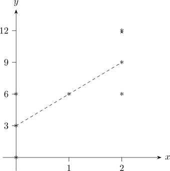
(b). The regression line. \[b=\frac {S_{xy}}{S_{xx}}=\frac {18}{6}=3,\qquad a=\overline {y}-b\overline {x}=6-3(1)=3,\] \[\hat {y}=3+3x.\]
- \(\bullet \)
- The slope, \(b=3\): a one-unit increase in \(x\) is associated with an increase of \(3\) units in \(y\) on average.
- \(\bullet \)
- The intercept, \(a=3\): the predicted value of \(y\) when \(x=0\). Here — unlike the previous problem — \(x=0\) is genuinely in the data, three times over, so the intercept does mean something. The three observed values at \(x=0\) are \(0\), \(3\) and \(6\), whose mean is exactly \(3\).
(c). Testing for a positive linear relationship. \[SS_{\text {Regression}}=bS_{xy}=3(18)=54,\qquad SS_{\text {Error}}=90-54=36,\] \[\hat {\sigma }^2=\frac {36}{n-2}=\frac {36}{5}=7.2,\qquad \hat {\sigma }=2.683,\] \[\text {S.E}(b)=\frac {\hat {\sigma }}{\sqrt {S_{xx}}}=\frac {2.683}{\sqrt {6}}=1.095.\]
- 1.
- \(H_0:\ \beta =0\); \(H_1:\ \beta >0\) — “positive” is directional, so one-tailed.
- 2.
- \(\alpha =0.01\).
- 3.
- \(t=\dfrac {3}{1.095}=2.74\) on \(n-2=5\) degrees of freedom.
- 4.
- Critical region: \(t_{5,\,0.01}=3.365\), so reject if \(t>3.365\).
- 5.
- \(2.74<3.365\), so we fail to reject \(H_0\). At the \(1\%\) level there is no evidence of a positive linear relationship.
(d). Confidence interval for \(\beta \). With \(t_{5,\,0.005}=4.032\), \[3\pm 4.032(1.095)=3\pm 4.42\quad \implies \quad -1.42<\beta <7.42.\] The interval contains zero, agreeing with (c).
(e). Correlation coefficient. \[r=\frac {S_{xy}}{\sqrt {S_{xx}S_{yy}}}=\frac {18}{\sqrt {6(90)}}=\frac {18}{\sqrt {540}} =\frac {18}{23.24}=0.775.\]
This problem is a useful counterweight to the last one. There \(r=-0.892\) and the slope was decisively significant; here \(r=0.775\), which still sounds like a strong correlation, and yet the slope cannot be distinguished from zero. Three things explain the difference: only seven observations rather than nine; only three distinct values of \(x\), which makes \(S_{xx}=6\) against \(375\) and so inflates the standard error of the slope; and a much stricter one-tailed test at \(1\%\). A large \(r\) is not by itself evidence of a relationship — what matters is \(r\) judged against the sample size and the spread of the \(x\) values, and that judgement is exactly what the \(t\)-test performs.
Questions on this section
Stuck on something here? Ask below and it stays attached to this topic.