5.5 Inference for the Regression Line
Fitting a line is only half the work. Least squares will happily draw a line through points with no relationship whatever, so the next question is whether the slope we obtained is real or could plausibly have arisen by chance.
5.5.1 Partitioning the variation
Exactly as in the analysis of variance, the total variation in \(Y\) splits into a part the line explains and a part it does not: \[\underbrace {\sum (Y_i-\overline {Y})^2}_{SS_T} =\underbrace {\sum (\hat {Y}_i-\overline {Y})^2}_{SS_R\ \text {(regression)}} +\underbrace {\sum (Y_i-\hat {Y}_i)^2}_{SS_E\ \text {(error)}}\] where \(\hat {Y}_i=\hat {a}+\hat {b}X_i\) is the value the line predicts. \(SS_E\) is the sum of squared residuals – the vertical gaps between the points and the line, which is precisely the quantity least squares chose \(\hat {a}\) and \(\hat {b}\) to make as small as possible.
5.5.2 The coefficient of determination
Definition 5.5. The coefficient of determination is \[R^2=\frac {SS_R}{SS_T}=1-\frac {SS_E}{SS_T},\] the proportion of the variation in \(Y\) that the regression line accounts for.
\(R^2\) lies between 0 and 1, and in simple linear regression it is exactly the square of the correlation coefficient, \(R^2=r^2\). An \(R^2\) of \(0.81\) says the line accounts for \(81\%\) of the variation in \(Y\); the remaining \(19\%\) is unexplained.
Two warnings. A high \(R^2\) does not mean the straight-line model is right – data curving in a smooth arc can produce a large \(R^2\) while a straight line is plainly the wrong shape, which is why the residuals should always be plotted. And \(R^2\) says nothing about causation: \(X\) may predict \(Y\) well without influencing it at all.
5.5.3 The ANOVA table for regression
| Source | \(SS\) | df | \(MS\) | \(F\) |
| Regression | \(SS_R\) | \(1\) | \(MS_R=\frac {SS_R}{1}\) | \(\frac {MS_R}{MS_E}\) |
| Error | \(SS_E\) | \(n-2\) | \(MS_E=\frac {SS_E}{n-2}\) | |
| Total | \(SS_T\) | \(n-1\) |
The degrees of freedom are worth reading rather than memorising. The total carries \(n-1\), one lost to estimating \(\overline {Y}\). The regression carries \(1\), because a straight line has one slope. The error carries \(n-2\), since fitting the line used up two estimates, \(\hat {a}\) and \(\hat {b}\) – and \(1+(n-2)=n-1\), so the table balances.
Under \(H_0:\beta =0\) the ratio \(F=MS_R/MS_E\) follows an \(F\) distribution with \(1\) and \(n-2\) degrees of freedom. A large \(F\) is evidence that the line explains more than chance would.
5.5.4 Testing and estimating the slope
The quantity \(MS_E\) estimates \(\sigma ^2\), the variance of the errors about the line, and its square root \(s=\sqrt {MS_E}\) is the standard error of the estimate. The standard error of the slope is \[SE(\hat {b})=\frac {s}{\sqrt {\sum (X_i-\overline {X})^2}}.\] The denominator carries a useful message: the more spread out the \(X\) values, the smaller the standard error. A line is pinned down more firmly by observations taken over a wide range of \(X\) than by the same number bunched together.
To test \(H_0:\beta =0\) against \(H_1:\beta \neq 0\), use \[t=\frac {\hat {b}-0}{SE(\hat {b})}, \qquad \text {df}=n-2,\] and reject when the \(P\)-value is below \(\alpha \). In simple linear regression this \(t\)-test and the \(F\)-test above always agree, because \(t^2=F\) – they are the same test written two ways.
A confidence interval for the slope is \[\hat {b}\pm t_{n-2,\,\alpha /2}\times SE(\hat {b}),\] and for the intercept \[\hat {a}\pm t_{n-2,\,\alpha /2}\times s\sqrt {\frac {1}{n}+\frac {\overline {X}^2}{\sum (X_i-\overline {X})^2}}.\] Both use \(t\) with \(n-2\) degrees of freedom, by the rule from the previous chapter: \(\sigma \) is unknown and has been estimated from the data.
The interval for the slope is often more informative than the test. If it excludes zero we would reject \(H_0\)
at that level anyway – but the interval also shows how large the effect might plausibly be, which a
\(P\)-value alone never does.
The regression line will pass through the point \((\overline {X},\overline {Y})\).
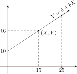
substituting in the Regression line \(\hat {Y}\)- predicted value gives \(X=25\).
| \(X\) | 0.1 | 0.2 | 0.3 | 0.4 | 0.5 | 0.6 | 0.7 | 0.8 | 0.9 | 1.0 |
| \(Y\) | 10.7 | 11.3 | 12.0 | 12.4 | 13.0 | 13.7 | 14.5 | 15.1 | 15.6 | 16 |
Find the regression line \(Y=\hat {a}+\hat {b}X\)
Solution.
| \(X\) | \(Y\) | \(XY\) | \(X^2\) | \((Y-\hat {Y})^2\) |
| 0.1 | 10.7 | |||
| 0.2 | 11.3 | |||
| 0.3 | 12.0 | |||
| 0.4 | 12.4 | |||
| 0.5 | 13.0 | |||
| 0.6 | 13.7 | |||
| 0.7 | 14.5 | |||
| 0.8 | 15.1 | |||
| 0.9 | 15.6 | |||
| 1.0 | 16.0 | |||
| 5.5 | 134.4 | 78.88 | 3.85 | 0.11784 |
\begin {align*} \hat {b} &=\frac {n\sum XY-\sum X\sum Y}{n\sum X^2-\Bigg (\sum X\Bigg )^2}\hspace {0.5cm}\implies \hspace {0.5cm} \hat {b}=6.08\\\\ \hat {a}&=10.1\\ \end {align*}
\(\therefore \hspace {0.3cm}\) The regression line of \(Y\) on \(X\) is \(Y=10.1+6.08X\)
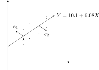
The interpretation of \(\hat {b}=6.08\). This is the expected change in length of the spring with 1 unit increase in
weight\((X)\).
If \(X=17\), what is the expected value of \(Y\)?
\[\mu _{Y(X=17)}=10.1+6.08\times 17\]
If \(X=18\), what is \(P(Y>20)\)?
\[P(Y>20| X=18)=P\Bigg (\frac {20-18}{\sigma }\Bigg )=1-P(Z<Z_1)\]
The predicted values from the regression line is \(\hat {Y}=\hat {a}+\hat {b}X\).
If \(X=1.2\implies \hat {Y}=10.1+6.08\times 1.2\)
\(\hat {Y}=17.4\), this is the predicted value for \(X=1.2\)
\begin {align*} \hat {Y}_i &=\hat {a}+\hat {b}X_i\\\\ \hat {Y}_1 &=\hat {a}+\hat {b}X_1\\ \hat {Y}_2 &=\hat {a}+\hat {b}X_2\\ .\\ .\\ .\\ \hat {Y}_n &=\hat {a}+\hat {b}X_n\\ \end {align*}
\(*\) Residuals are deviations of observed and predicted values
\[\text {SSE}=\sum _i^ne_i^2=\sum (Y-\hat {Y})^2\]
Which in turn allows us to estimate \(\theta ^2\).
As well as an important statistics referred to as the coefficients of determination
\[R^2=1-\frac {\text {SSE}}{\text {SST}},\hspace {1cm} \text {SST}=\sum ^n_i(Y-\hat {Y})^2\]
5.5.5 Estimating A Value for \(\sigma ^2_{Y/X}\)
For a value of \(X\) the value of \(Y\). Predicting by the regression line is given by \(\hat {Y}=\hat {a}+\hat {b}X\).
The difference between \(Y\) and \(\hat {Y}\) is known as a residual, gives the value of \(e\) for that point.
Each value of \(\hat {Y}-Y\) gives value of \(e_i\) from a distribution which is \(N(0,\sigma ^2_{Y/X})\). The unbiased estimate\(\hat {S}_{Y/X}\) is given
by
\[\hat {S}_{Y/X}=\sqrt {\frac {\sum (\hat {Y}-Y)^2}{n-2}}\]
\(n-2\) is the df, \(\hat {a}\), \(\hat {b}\) are calculated from the values of \(X\) and \(Y\).
Example 5.7. Obtain an estimate of \(\sigma ^2_{Y/X}\) for the examination marks above, and use it to find \(P(Y>90 \mid X=80)\).
Solution. From \(S_{XY}=3412.4\) and \(S_{XX}=3584.4\), \[\hat {b}=\frac {S_{XY}}{S_{XX}}=0.952,\qquad \hat {a}=\overline {Y}-\hat {b}\,\overline {X}=57.1-0.952(56.6)=3.22,\] so the fitted line is \(\hat {Y}=3.22+0.952X\).
Summing the squared residuals gives \(\sum (Y-\hat {Y})^2=988.25\), so \[\hat {S}_{Y/X}=\sqrt {\frac {\sum (Y-\hat {Y})^2}{n-2}}=\sqrt {\frac {988.25}{8}} =\sqrt {123.53}=11.11.\] The divisor is \(n-2\) because two parameters, \(\hat {a}\) and \(\hat {b}\), were estimated before the residuals could be formed.
For a candidate scoring \(X=80\) on Paper 1, the predicted Paper 2 mark is \[\hat {Y}=3.22+0.952(80)=79.4,\] and the residuals are taken to be \(N(0,\sigma ^2_{Y/X})\). Hence \[P(Y>90 \mid X=80)=P\left (Z>\frac {90-79.4}{11.11}\right )=P(Z>0.95)=1-0.8289=0.171.\] So about \(17\%\) of candidates scoring \(80\) on Paper 1 would be expected to exceed \(90\) on Paper 2.
Note how much wider this is than the line alone suggests. The regression gives a single predicted value, \(79.4\); the residual standard deviation of \(11.11\) is what says how far an individual candidate may sit from it. A prediction without \(\hat {S}_{Y/X}\) beside it claims a precision the data do not support.
5.5.6 Confidence Limit For \(\beta \)
How accurate is the estimate \(\hat {b}\) which we have made of \(\beta \)? Here we want the limit of \(\beta \) in terms \(\sigma _{Y/X}\) the s.d. of
the random error \(e_i\).
we assume with a normal distribution with mean 0 and s.d. \(\sigma _{Y/X}\).
\[E(e)=0\hspace {1cm}\text {and}\hspace {1cm} \text {var}(e)=\sigma ^2_{Y/X}\]
We want to calculate the expected value and variance of \(\hat {b}\) in terms of \(e_i\)
\begin {align*} \hat {b} &=\frac {n\sum XY-\sum X\sum Y}{n\sum X^2-\Bigg (\sum X\Bigg )^2}\\\\ \implies &Y=\alpha +\beta X +e\\ \end {align*}
\(Y=\beta X+\alpha e\) substitute in \[\hat {b}=\frac {n\sum X(\beta X+\alpha +e)-\sum X\sum (\beta X+\alpha +e)}{n\sum X^2-\Bigg (\sum X\Bigg )^2}\] Take the numerator
\begin {align*} &n\sum X(\beta X+\alpha +e)-\sum X\sum (\beta X+\alpha +e)\\\\ &= n\beta \sum X^2+n\alpha \sum X +n\sum Xe-\Bigg [\beta \Bigg (\sum X\Bigg )^2+\alpha n\sum X +\sum X\sum e\Bigg ]\\\\ &=\beta \Bigg [n\sum X^2-\Bigg (\sum X\Bigg )^2\Bigg ]+n\sum Xe-\frac {n}{n}\sum X\sum e\\\\ &=\beta \Bigg [n\sum X^2-\Bigg (\sum X\Bigg )^2\Bigg ] +n\sum Xe-n\overline {X}\sum e\\\\ &=\beta \Bigg [n\sum X^2-\Bigg (\sum X\Bigg )^2\Bigg ]+n\sum (X-\overline {X})e\\ \end {align*}
Dividing the denominator in \(\hat {b}\) \begin {align*} \hat {b} &=\frac {\beta \Bigg [n\sum X^2-\Bigg (\sum X\Bigg )^2\Bigg ]+n\sum (X-\overline {X})e}{n\sum X^2-\Bigg (\sum X\Bigg )^2}\\\\ &=\beta +\frac {n\sum (X-\overline {X})e}{n\sum X^2-\Bigg (\sum X\Bigg )^2}\\\\ &=\beta +\frac {n\sum (X-\overline {X})e}{n\sum (X-\overline {X})^2}\\\\ \implies \hspace {0.5cm} \hat {b}&=\beta +\frac {\sum (X-\overline {X})e_i}{\sum (X-\overline {X})^2} \end {align*}
In this calculation the expected value and variance of \(\hat {b}\).
The terms in \(X_i\) is constant \((X_1-\overline {X}, X_2-\overline {X}, \ldots , X_i-\overline {X})\) for each \(e_i\) since the value of \(X_i\) are pre-determined
\begin {align*} E(\hat {b}) &=\beta +\frac {E\Bigg (\sum (X-\overline {X})e_i\Bigg )}{\sum (X-\overline {X})^2}\\\\ &=\beta +\frac {\sum (X-\overline {X})E(e)}{\sum (X-\overline {X})^2}\\\\ & But \hspace {0.5cm} E(e)=0\\ \end {align*}
\(\implies \hspace {0.5cm} E(\hat {b})=\beta \hspace {0.4cm}\) \(\hat {b}\) is an unbiased estimator of \(\beta \).
\begin {align*} \text {var}(\hat {b}) &=\text {var}\Bigg [\frac {\sum (X-\overline {X})e}{\sum (X-\overline {X})^2}\Bigg ]\hspace {0.5cm}\implies \hspace {0.5cm} \text {var}(\hat {b})=\frac {\sum (X-\overline {X})^2\sum e_i}{\Bigg [\sum (X-\overline {X})^2\Bigg ]^2}\\ \text {aX}&=a\text {var}(X)\\\\ \text {var}(X) &=\frac {\sigma ^2_{Y/X}}{\sum (X-\overline {X})^2}\\ \end {align*}
Assuming the sampling distribution of \(\hat {b}\) is normal the \(95\%\) C.I of \(\beta \) is given by
\[\beta =\hat {b}\pm \frac {Z_{\alpha /2}\times \sigma _{Y/X}}{\sqrt {\sum (X-\overline {X})^2}}\hspace {0.5cm}\text {If}\hspace {0.3cm}\sigma _{Y/X}^2\hspace {0.3cm} \text {is known}.\]
\[\beta =\hat {b}\pm \frac {t_{n-2,\alpha /2}\times \hat {S}_{Y/X}}{\sqrt {\sum (X-\overline {X})^2}}\hspace {1cm} \text {if}\hspace {0.3cm}\sigma ^2_{Y/X}\hspace {0.3cm}\text {is estimated from}\hspace {0.3cm} \hat {S}_{Y/X}\]
Example 5.8. For the examination marks above, calculate a \(95\%\) confidence interval for \(\beta \).
Solution. \(\sigma _{Y/X}\) is not known – it has been estimated by \(\hat {S}_{Y/X}\) – so the multiplier is \(t\) with \(n-2=8\) degrees of freedom: \[\beta =\hat {b}\pm t_{n-2,\,\alpha /2}\times \frac {\hat {S}_{Y/X}}{\sqrt {\sum (X-\overline {X})^2}}.\] Note the square in \(\sum (X-\overline {X})^2\); this is \(S_{XX}\), and \(\sum (X-\overline {X})\) would be zero.
With \(\hat {b}=0.952\), \(\hat {S}_{Y/X}=11.11\), \(S_{XX}=3584.4\) and \(t_{8,\,0.025}=2.306\): \[SE(\hat {b})=\frac {11.11}{\sqrt {3584.4}}=\frac {11.11}{59.87}=0.186,\] \[\beta =0.952\pm 2.306(0.186)=0.952\pm 0.428.\] So we are \(95\%\) confident that the true slope lies between \[0.952-0.428=0.524 \qquad \text {and}\qquad 0.952+0.428=1.380.\]
The interval excludes zero, so there is evidence of a real linear relationship – the same conclusion the \(t\)-test reaches, since \(t=0.952/0.186=5.13\) against a critical \(2.306\).
But the interval says more than the test does. A slope anywhere from \(0.52\) to \(1.38\) is consistent with these data: a mark on Paper 1 might be worth only half a mark on Paper 2, or nearly one and a half. Ten candidates simply cannot pin it down more tightly than that, and reporting only “significant” would conceal how wide the uncertainty remains.
Questions on this section
Stuck on something here? Ask below and it stays attached to this topic.