1.11 Percentiles
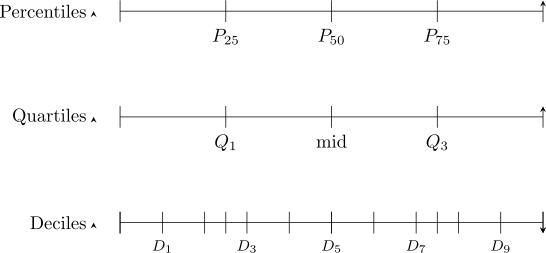
Quartiles cut ordered data into four equal parts. Percentiles do the same thing more finely, cutting it into a hundred.
Definition 1.41. The \(k\)th percentile \(P_k\) is the value below which \(k\) per cent of the ordered observations lie.
So \(P_{25}\), \(P_{50}\) and \(P_{75}\) are the lower quartile, the median and the upper quartile respectively, and \(P_{50}=Q_2=\text {median}\). Deciles cut the data into ten, so \(D_6=P_{60}\).
Finding a percentile. Order the data, then locate the position \[\text {position of }P_k=\frac {k}{100}\times n.\] If that position is not a whole number, the value lies between the two observations either side of it; take their average.
Example 1.42. For the eleven ordered values \[3,\ 5,\ 8,\ 9,\ 12,\ 14,\ 15,\ 18,\ 20,\ 24,\ 30\] find \(P_{25}\), the median, and \(P_{80}\).
Solution. Here \(n=11\).
\(P_{25}\) lies at position \(\tfrac {25}{100}\times 11=2.75\), that is between the 2nd and 3rd values, \(5\) and \(8\): \[P_{25}=\frac {5+8}{2}=6.5.\]
The median is \(P_{50}\), at position \(\tfrac {50}{100}\times 11=5.5\), between the 5th and 6th values, \(12\) and \(14\): \[P_{50}=\frac {12+14}{2}=13.\]
\(P_{80}\) lies at position \(\tfrac {80}{100}\times 11=8.8\), between the 8th and 9th values, \(18\) and \(20\): \[P_{80}=\frac {18+20}{2}=19.\] So \(80\%\) of the observations fall below \(19\).
Remark 1.43. Percentiles are what make otherwise meaningless numbers comparable. A mark of \(62\) says nothing on its own; that it sits at \(P_{90}\) says a great deal. This is why examination results, growth charts and test scores are so often reported as percentiles rather than as raw values.
Be aware that textbooks and software differ slightly in how they handle a non-integer position – some interpolate between the neighbouring values rather than averaging them, so answers can disagree in the last figure. This course uses the position method above throughout.
Take the assumed mean at the middle class, \(a=25\), with class width \(h=10\). Write \(D=X-a\) and \(U=\frac {X-a}{h}\).
| C-I | \(f\) | \(X\) | \(D=X-a\) | \(fD\) | \(fD^2\) | \(U\) | \(fU\) | \(fU^2\) |
| \(0-10\) | 5 | 5 | \(-20\) | \(-100\) | 2000 | \(-2\) | \(-10\) | 20 |
| \(10-20\) | 10 | 15 | \(-10\) | \(-100\) | 1000 | \(-1\) | \(-10\) | 10 |
| \(20-30\) | 15 | 25 | 0 | 0 | 0 | 0 | 0 | 0 |
| \(30-40\) | 5 | 35 | 10 | 50 | 500 | 1 | 5 | 5 |
| \(40-50\) | 5 | 45 | 20 | 100 | 2000 | 2 | 10 | 20 |
| Total | 40 | \(-50\) | 5500 | \(-5\) | 55 |
From the \(D\) columns, \[\overline {X}=a+\frac {\sum fD}{\sum f}=25+\frac {-50}{40}=23.75,\] \[\sigma ^2=\frac {\sum fD^2}{\sum f}-\left (\frac {\sum fD}{\sum f}\right )^{2} =\frac {5500}{40}-(-1.25)^2=137.5-1.5625=135.94,\] so \(\sigma =\sqrt {135.94}=11.66\).
The \(U\) columns give the same answers with smaller numbers, which is the whole reason for the substitution: \[\overline {X}=a+h\,\frac {\sum fU}{\sum f}=25+10\left (\frac {-5}{40}\right )=23.75,\] \[\sigma ^2=h^2\left [\frac {\sum fU^2}{\sum f}-\left (\frac {\sum fU}{\sum f}\right )^{2}\right ] =100\left [\frac {55}{40}-\left (\frac {-5}{40}\right )^{2}\right ]=100(1.359375)=135.94.\] Dividing by \(h\) before squaring keeps the arithmetic to single digits; multiplying back by \(h^2\) at the end restores the scale. With a hand calculation over many classes that is a real saving, and it is exactly why the coded method exists.
1.11.1 The five working forms of the variance
These are five ways of writing the same quantity. They always give the same answer; which one is least work depends on what the data looks like.
- 1.
- From the definition, grouped data. Every deviation must be computed separately, which is why the forms below exist. \[\sigma ^2=\frac {\sum f(X-\overline {X})^2}{\sum f}\]
- 2.
- Raw scores. Expanding the square trades the deviations for two running totals, \(\sum X\) and \(\sum X^2\). \[\sigma ^2=\frac {\sum X^2}{n}-\Bigg (\frac {\sum X}{n}\Bigg )^{2}\]
- 3.
- Raw scores with frequencies. The same identity when values repeat. \[\sigma ^2=\frac {\sum fX^2}{\sum f}-\Bigg (\frac {\sum fX}{\sum f}\Bigg )^{2}\]
- 4.
- Deviations from an assumed mean, \(D_X=X-a\). Shifting the origin does not change a variance, so \(a\) may be chosen to make the numbers small. \[\sigma ^2=\frac {\sum fD_X^{2}}{\sum f}-\Bigg (\frac {\sum fD_X}{\sum f}\Bigg )^{2}\]
- 5.
- Coded deviations, \(U_X=\frac {X-a}{h}\), where \(h\) is the class width. Dividing by \(h\) scales the variance by \(h^2\), which is put back at the end. \[\sigma ^2=\Bigg [\frac {\sum fU_X^{2}}{\sum f}-\Bigg (\frac {\sum fU_X}{\sum f}\Bigg )^{2}\Bigg ]h^{2}\]
Form 2 is the one worth being able to derive; forms 3 to 5 follow from it in the same way.
Proof. \begin {align*} \sigma ^2 &= E(X-\overline {X})^2=\frac {1}{n}\sum (X-\overline {X})^2 =\frac {1}{n}\sum \left (X^2-2X\overline {X}+\overline {X}^2\right )\\ &=\frac {1}{n}\Bigg (\sum X^2-2\overline {X}\sum X +\sum \overline {X}^2\Bigg )\\ &=\frac {1}{n}\Bigg [\sum X^2-2n\overline {X}^2+n\overline {X}^2\Bigg ]\\ &=\frac {1}{n}\sum X^2-\overline {X}^2\\ &=\frac {\sum X^2}{n}-\Bigg (\frac {\sum X}{n}\Bigg )^{2}. \end {align*} □
The two middle steps are where it is usually got wrong. \(\overline {X}\) is a constant, so it comes outside the sum; and \(\sum X=n\overline {X}\), which is what turns the middle term into \(2n\overline {X}^2\).
Questions on this section
Stuck on something here? Ask below and it stays attached to this topic.