13.2 The instrumental variables estimator

Definition 13.2.1. In the model $Y = X\beta + U$ with $X$ of order $n \times k$, an $n \times \ell $ matrix $Z$ of instruments, with $\ell \geq k$, satisfies

(i): exogeneity: $\plim \frac 1nZ'U = 0$;
(ii): relevance: $\plim \frac 1nZ'X = Q_{ZX}$ has rank $k$;

together with $\plim \frac 1nZ'Z = Q_{ZZ}$ positive definite. The exogenous columns of $X$, including the constant, serve as their own instruments, so $Z$ contains them. The equation is exactly identified if $\ell = k$ and overidentified if $\ell > k$.

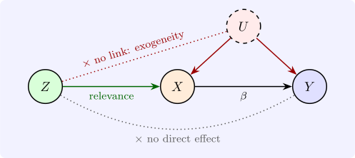
ZXYUrβ××elennvooan l dciniekre:c etx eoffgeecnteity — Figure 14: The logic of an instrument. $U$ affects both $X$ and $Y$, so the association between them mixes $\beta $ with the effect of $U$. The instrument $Z$ moves $X$ but is unrelated to $U$ and affects $Y$ only through $X$; the part of the variation in $X$ that comes from $Z$ is therefore free of $U$, and identifies $\beta $.

Condition (ii) for $\ell = k$ says that $Z'X$ is non-singular; it requires at least as many excluded instruments as endogenous regressors (the order condition), and that they be correlated with the endogenous regressors in a non-degenerate way (the rank condition).

Theorem 13.2.2. If $\ell = k$, the instrumental variables (IV) estimator \[ b_{\text {IV}} = (Z'X)^{-1}Z'Y \] is consistent for $\beta $. If moreover the rows $(z_i', u_i)$ are independent with $E(u_i^2 \mid z_i) = \sigma ^2$, then \[ \sqrt n(b_{\text {IV}} - \beta ) \xrightarrow {d} N\bigl (0,\ \sigma ^2Q_{ZX}^{-1}Q_{ZZ}Q_{XZ}^{-1}\bigr ), \qquad Q_{XZ} = Q_{ZX}' , \] and $\sigma ^2$ is estimated consistently by $s^2 = \hat u'\hat u/(n - k)$ with $\hat u = Y - Xb_{\text {IV}}$.

Proof. $b_{\text {IV}} = (Z'X)^{-1}Z'(X\beta + U) = \beta + \bigl (\frac 1nZ'X\bigr )^{-1}\frac 1nZ'U$. The first factor converges to $Q_{ZX}^{-1}$ and the second to zero, so $b_{\text {IV}} \xrightarrow {p} \beta $ by Slutsky’s theorem. For the distribution, $\frac {1}{\sqrt n}Z'U = \frac {1}{\sqrt n}\sum z_iu_i$ is a scaled sum of independent vectors with mean zero and variance $E(u_i^2z_iz_i') = \sigma ^2E(z_iz_i')$, so it converges to $N(0, \sigma ^2Q_{ZZ})$ by the central limit theorem. Multiplying by $Q_{ZX}^{-1}$ gives the stated variance. For $s^2$, $\hat u = U - X(b_{\text {IV}} - \beta )$, and $\frac 1n\hat u'\hat u = \frac 1nU'U - 2\frac 1nU'X(b_{\text {IV}} - \beta ) + (b_{\text {IV}} - \beta )'\frac 1nX'X(b_{\text {IV}} - \beta ) \xrightarrow {p} \sigma ^2$, since $b_{\text {IV}} - \beta \xrightarrow {p} 0$. □

In the two-variable case with a single instrument, in deviations, \[ b_{\text {IV}} = \frac {\sum z_iy_i}{\sum z_ix_i}, \qquad \frac {\text {asymptotic variance of } b_{\text {IV}}}{\text {asymptotic variance of } b} = \frac {1}{r_{xz}^2}, \] where $r_{xz}$ is the correlation between $x$ and $z$, when both estimators are consistent. The price of consistency is precision, and it is high when the instrument is only weakly correlated with the regressor: with $r_{xz} = 0.3$ the IV standard error is more than three times that of least squares.

Example 13.2.3. With a binary instrument $z_i \in \{0, 1\}$, the IV slope is the Wald estimator \[ b_{\text {IV}} = \frac {\bar y_1 - \bar y_0}{\bar x_1 - \bar x_0}, \] the difference in mean outcomes between the two instrument groups divided by the difference in mean regressor. (In deviations $\sum (z_i - \bar z)y_i = n_1(\bar y_1 - \bar y)$ and $\bar y_1 - \bar y = \frac {n_0}{n}(\bar y_1 - \bar y_0)$, and likewise for $x$.) Angrist (1990) used the Vietnam draft lottery as the instrument for military service. With illustrative round numbers: if men with low lottery numbers earned $900 less a year and were $16$ percentage points more likely to have served, the IV estimate of the effect of service is $-900/0.16 = -\$5\,625$ a year. The instrument is credible because the lottery number was random, and so unrelated to anything else that affects earnings.

[next] [prev] [prev-tail] [front] [up]

Questions on this section

Stuck on something here? Ask below and it stays attached to this topic.