9.3 Fitted Values and Residuals
Using the least squares estimates \(\widehat {B}\) we can form the matrices of predicted values \begin {equation} \tag {7} \widehat {Y} = Z\widehat {B} = Z\big (Z'Z\big )^{-1}Z'Y \end {equation}
\begin {align*} \text {Residuals}:\quad \widehat {\varepsilon } & = Y - \widehat {Y}\\ & = Y - Z\big (Z'Z\big )^{-1}Z'Y\\ & = \big [I- Z\big (Z'Z\big )^{-1}Z'\big ]Y\\ & = HY\tag {8} \end {align*}
The orthogonality conditions among the residuals, predicted values and columns of \(Z\) which hold in classical regression hold in multivariate regression. Specifically we have the following
- (1).
- \begin {align*} Z'H & = Z'\big (I-Z\big (Z'Z\big )^{-1}Z'\big )\\ & = Z'- Z'Z\big (Z'Z\big )^{-1}Z'\\ & = Z'-Z'\\ & = \underline {0} \qquad \text {matrix} \end {align*}
- (2).
- \(Z'\widehat {\varepsilon } = Z'HY = OY =0\)
Two (2) says that the residuals \(\widehat {\varepsilon }_{(i)}\) are perpendicular to the columns of \(Z\). - (3).
- \(\widehat {Y}'\widehat {\varepsilon } = \widehat {B}'Z'\big [I-Z\big (Z'Z\big )^{-1}Z'\big ]Y=\widehat {B} 0 =0\).
(3) this confirms that the predicted values \(Y_{(i)}\) are perpendicular to the residuals \(\widehat {\varepsilon }_{(k)}\).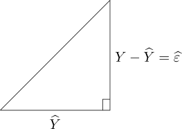
\begin {align*} \text {Now}\qquad Y & = \widehat {Y} + \widehat {\varepsilon }\\ Y'Y & = \big (\widehat {Y}+\widehat {\varepsilon }\big )'\big (\widehat {Y}+\widehat {\varepsilon }\big )\\ & = \widehat {Y}'\widehat {Y} + \widehat {Y}'\widehat {\varepsilon } + \widehat {\varepsilon }'\widehat {Y} + \widehat {\varepsilon }'\widehat {\varepsilon }\\ & = \widehat {Y}'\widehat {Y} + 0 + 0 + \widehat {\varepsilon }'\widehat {\varepsilon }\\ Y'Y & = \widehat {Y}'\widehat {Y} + \widehat {\varepsilon }'\widehat {\varepsilon }\tag {9} \end {align*}
\(Y'Y=\) Total sum of squares and cross products.
\(\widehat {Y}'\widehat {Y}=\) Predicted sum of squares and cross products.
\(\widehat {\varepsilon }'\widehat {\varepsilon } =\) Residual (error) sum of squares and cross products.
The residual sum of squares and cross products can also be written as \begin {equation} \tag {10} \widehat {\varepsilon }'\widehat {\varepsilon } = Y'Y-\widehat {Y}'\widehat {Y}= \widehat {B}'Z'Z\widehat {B} \end {equation}
Example 9.1. Illustrate the calculations of \(\widehat {B}\) and \(\widehat {Y}\) and \(\widehat {\varepsilon }\) we fit a straight line \begin {align*} y_{j1} & = \beta _{01} + \beta _{11}Z_{j1} + \varepsilon _{j1}\\ y_{j2} & = \beta _{02} + \beta _{12}Z_{j1} + \varepsilon _{j2}\qquad j=1,2,3,4,5 \end {align*}
| \(Z_1\) | 0 | 1 | 2 | 3 | 4 |
| \(Y_1\) | 1 | 4 | 3 | 8 | 9 |
| \(Y_2\) | \(-1\) | \(-1\) | 2 | 3 | 2 |
the design matrix \(Z\) remains unchanged of the single respect problem. \[ Z' = \begin {bmatrix} 1 & 1 & 1 & 1 & 1\\ 0 & 1 & 2 & 3 & 4\\ \end {bmatrix} \qquad \big (Z'Z\big )^{-1}= \begin {pmatrix} 5 & 10\\ 10 & 30\\ \end {pmatrix} \]
\[\big (Z'Z\big )^{-1} = \begin {pmatrix} 0.6 & -0.2\\ -0.2 & 0.1\\ \end {pmatrix} \]
\begin {align*} Z'Y_{(1)} & = \begin {pmatrix} 1 & 1 & 1 & 1 & 1\\ 0 & 1 & 2 & 3 & 4\\ \end {pmatrix} \begin {pmatrix} 1 \\ 4\\ 3\\ 8\\ 9\\ \end {pmatrix}\\ & = \begin {pmatrix} 25\\ 70\\ \end {pmatrix}\\ \end {align*}
\begin {align*} \text {So}\qquad \widehat {B}_{(1)} & = \big (Z'Z\big )^{-1}Z'Y_{(1)}\\ & = \begin {pmatrix} 0.6 & -0.2\\ -0.2 & 0.1\\ \end {pmatrix} \begin {pmatrix} 25\\70\\ \end {pmatrix}\\ & = \begin {pmatrix} 1\\2\\ \end {pmatrix}\\\\ \end {align*}
\[Z'Y_{(2)} = \begin {pmatrix} 1 & 1 & 1 & 1 & 1\\ 0 & 1 & 2 & 3 & 4\\ \end {pmatrix} \begin {pmatrix} -1 \\ -1 \\ 2\\ 3\\ 2\\ \end {pmatrix} = \begin {pmatrix} 5\\20\\ \end {pmatrix} \]
\begin {align*} \text {So}\qquad \widehat {B}_{(2)} & = \big (Z'Z\big )^{-1}Z'Y_{(2)}\\ & = \begin {pmatrix} 0.6 & -0.2\\ -0.2 & 0.1\\ \end {pmatrix} \begin {pmatrix} 5\\ 20\\ \end {pmatrix}\\ & = \begin {pmatrix} -1\\ 1\\ \end {pmatrix}\\\\ \end {align*}
\begin {align*} \widehat {B} & = \begin {bmatrix} \widehat {B}_{(1)} & \vdots & \widehat {B}_{(2)}\\ \end {bmatrix}\\ & = \begin {pmatrix} 1 & -1\\ 2 & 1\\ \end {pmatrix} =\big (Z'Z\big )^{-1}Z'Y\\ & = \big (Z'Z\big )^{-1}Z' \begin {pmatrix} Y_{(1)} & \vdots & Y_{(2)}\\ \end {pmatrix}\\ \end {align*}
\begin {align*} \text {Fitted equations}\qquad \widehat {Y}_1 & = 1 + 2Z_1\\ \widehat {Y}_2 & = -1 + Z_1\\ \end {align*}
\[\widehat {Y}=Z\widehat {B}= \begin {pmatrix} 1 & 0\\ 1 & 1\\ 1 & 2\\ 1 & 5\\ 1 & 4\\ \end {pmatrix} \begin {pmatrix} 1 & -1\\ 2 & 1\\ \end {pmatrix} =\begin {pmatrix} 1 & -1\\ 3 & 0\\ 5 & 1\\ 7 & 2\\ 9 & 3\\ \end {pmatrix} \]
\[\text {and}\qquad \widehat {\varepsilon } = Y - \widehat {Y}= \begin {pmatrix} 0 & 1 & -2 & 1 & 0\\ 0 & -1 & 1 & 1 & -1\\ \end {pmatrix}' \]
\[\widehat {\varepsilon }'\widehat {Y}= \begin {pmatrix} 0 & 1 & -2 & 1 & 0\\ 0 & -1 & 1 & 1 & -1\\ \end {pmatrix} \begin {pmatrix} 1 & -1\\ 3 & 0\\ 5 & 1\\ 7 & 2\\ 9 & 3\\ \end {pmatrix} = \begin {pmatrix} 0 & 0\\ 0 & 0\\ \end {pmatrix} \]
\[Y'Y = \begin {pmatrix} 1 & 4 & 3 & 8 & 9\\ -1 & -1 & 2 & 3 & 2\\ \end {pmatrix} \begin {pmatrix} 1 & -1\\ 4 & -1\\ 3 & 2\\ 8 & 3\\ 9 & 2\\ \end {pmatrix} = \begin {pmatrix} 171 & 43\\ 43 & 19\\ \end {pmatrix} \]
\[\widehat {Y}'\widehat {Y}= \begin {pmatrix} 165 & 45\\ 45 & 15\\ \end {pmatrix} \qquad \widehat {\varepsilon }'\widehat {\varepsilon }= \begin {pmatrix} 6 & -2\\ -2 & 4\\ \end {pmatrix} \]
Decomposition of sum of squares and cross-products is \(Y'Y = \widehat {Y}'\hat {Y} + \widehat {\varepsilon }'\widehat {\varepsilon }\)
\[ \begin {pmatrix} 171 & 43\\ 43 & 19\\ \end {pmatrix} = \begin {pmatrix} 165 & 45\\ 45 & 15\\ \end {pmatrix} + \begin {pmatrix} 6 & -2\\ -2 & 4\\ \end {pmatrix} \]
Result 9.2. For the least squares estimates \(\widehat {B} = \begin {bmatrix} \widehat {B}_{(1)} & \vdots & \widehat {B}_{(2)} & \vdots & \cdots& \widehat {B}_{(m)}\\ \end {bmatrix} \) determined under the multivariate multiple
regression model \(()\) with full \(rank(Z)=r+1<n\). \(E\big (\widehat {B}_{(i)}\big ) = B_{(i)}\) or \(E\big (\widehat {B}\big ) = B\) and \(cov\big (\widehat {B}_{(i)},\widehat {B}_{(k)}\big )=\sigma _{ik}\big (Z'Z\big )^{-1}, i,k=1,2,\ldots ,r+1\).
The residuals \( \widehat {\varepsilon } = \begin {bmatrix} \widehat {\varepsilon }_{(1)} & \vdots & \widehat {\varepsilon }_{(2)} & \vdots & \cdots& \vdots & \widehat {\varepsilon }_{(n)}\\ \end {bmatrix} =Y-Z\widehat {B}\) Satisfies \(E\big (\widehat {\varepsilon }_{(i)}\big )=\underline {0}\) and \(E\big (\widehat {\varepsilon }_{(i)}'\widehat {\varepsilon }_{(k)}\big )=(n-r-1)\sigma _{ik}\) as a result \(E\big (\widehat {\varepsilon }\big )=0\) and \[E\Bigg (\frac {\widehat {\varepsilon }'\widehat {\varepsilon }}{n-r-1}\Bigg )=\Sigma \]
Also \(\widehat {\varepsilon }\) and \(\widehat {B}\) are uncorrelated.
Proof. The \(i^{\text {th}}\) response follows the multiple regression model \[Y_{(i)}=ZB_{(i)}+\varepsilon _{(i)}, E\big (\varepsilon _{(i)}\big )=\underline {0}, E\big (\varepsilon _{(i)},\varepsilon _{(i)}'\big )=\sigma _{ii}I\] We also have: \begin {align*} \widehat {B}_{(i)} - B_{(i)} & = \big (Z'Z\big )^{-1}Z'Y_{(i)}-B_{(i)}\\ & = \big (Z'Z\big )^{-1}Z'\varepsilon _{(i)}\\ & = \big (Z'Z\big )^{-1}Z'\big (ZB_{(i)}+\varepsilon _{(i)}\big )-B_{(i)}\\ & = \big (Z'Z\big )^{-1}Z'ZB_{(i)} +\big (Z'Z\big )^{-1}Z'\varepsilon _{(i)}-B_{(i)}\\ & = B_{(i)} + \big (Z'Z\big )^{-1}\varepsilon _{(i)}-B_{(i)}\\ & = \big (Z'Z\big )^{-1}Z\varepsilon _{(i)}\\ \end {align*} □
\begin {align*} \text {and}\qquad \widehat {\varepsilon }_{(i)} & = Y_{(i)} - \widehat {Y}_{(i)}\\ & = Y_{(i)} - Z\widehat {B}_{(i)}\\ & = Y_{(i)} - Z\big (Z'Z\big )^{-1}Z'Y_{(i)}\\ & = \big (I-Z\big (Z'Z\big )^{-1}Z'\big )Y_{(i)}\\ & = \big (I-Z\big (Z'Z\big )^{-1}Z'\big )\varepsilon _{(i)} \end {align*}
So \(E\big (\widehat {B}_{(i)}=B_{(i)}\) since \begin {align*} E\big (\widehat {B}_{(i)}-B_{(i)}\big ) & = E\big [\big (Z'Z\big )^{-1}Z'\varepsilon _{(i)}\big ]\\ & = \big (Z'Z\big )^{-1}Z'\underline {0}\\ & = \underline {0}\\ \end {align*}
\begin {align*} E\big (\widehat {\varepsilon }_{(i)}\big ) & = E\big [\big (I-Z\big (Z'Z\big )^{-1}Z'\big )\varepsilon _{(i)}\big ]\\ & = \big (I-Z\big (Z'Z\big )^{-1}Z'\big )E\big (\varepsilon _{(i)}\big )\\ & = \big (I-Z\big (Z'Z\big )^{-1}Z'\big )\underline {0}\\ & = \underline {0}\\ \end {align*}
Next \begin {align*} Cov\big (\widehat {B}_{(i)},\widehat {B}_{(k)}\big ) & = E\big (\widehat {B}_{(i)}-B_{(i)}\big )\big (\widehat {B}_{(i)}-B_{(i)}\big )'\\ & = E\big [\big (Z'Z\big )^{-1}Z'\varepsilon _{(i)}\varepsilon '_{(k)}Z\big (Z'Z\big )^{-1}\big ]\\ & = \big (Z'Z\big )^{-1}Z'\sigma _{ik}IZ\big (Z'Z\big )^{-1}\\ & = \sigma _{ik}\big (Z'Z\big )^{-1}Z'Z\big (Z'Z\big )^{-1}\\ & = \sigma _{ik}\big (Z'Z\big )^{-1}\\ \end {align*}
If \(\underline {U}\) is any random vector and \(A\) is a fixed matrix then \begin {align*} E\big (U'AU\big ) & = E\big (tr\big (U'AU\big )\big )\\ & = E\big (tr(AUU'\big )\big )\\ & = tr\big (AE\big (UU'\big )\big ) \end {align*}
Using this result we have \begin {align*} E\big (\widehat {B}_{(i)}',\widehat {B}_{(k)}\big ) & = E\big (\varepsilon '_{(i)}\big (I-Z\big (Z'Z\big )^{-1}Z'\big )\varepsilon _{(k)}\big )\\ & = tr\big [\big (I-Z\big (Z'Z\big )^{-1}Z'\big )\sigma _{ik}I\big ]\\ & = \sigma _{ik}tr\big (I-Z\big (Z'Z\big )^{-1}Z'\big )\\ & = \sigma _{ik}\big [tr(I)-tr\big (Z\big (Z'Z\big )^{-1}Z'\big ]\\ & = \sigma _{ik}\big (n-tr\big [\big (Z'Z\big )^{-1}Z'Z\big ]\\ & = \sigma _{ik}\big (n-tr I_{r+1}\big )\\ & = \sigma _{ik}\big (n-(r+1)\big )\\ & = \sigma _{ik}(n-r-1)\\ \end {align*}
dividing each entry \(\widehat {\varepsilon }_{(i)}'\widehat {\varepsilon }_{(k)}\) of \(\widehat {\varepsilon }'\widehat {\varepsilon }\) by \(n-r-1\), we obtain the unbiased estimate of \(\Sigma \). Finally \(\big (\widehat {\varepsilon }_{(i)},\widehat {\varepsilon }_{(k)}\big ) = E\big [\big (Z'Z\big )^{-1}Z'\varepsilon _{(i)}\varepsilon _{(k)}'H\big ]\) where \begin {align*} H & = I- Z\big (Z'Z\big )^{-1}Z'\\ & = \big (Z'Z\big )^{-1}Z'\big (\varepsilon _{(i)}\varepsilon _{(k)}'\big )\big (I-Z\big (Z'Z\big )^{-1}Z'\big )\\ & = \big (Z'Z\big )^{-1}Z'\sigma _{ik}I\big (I-Z\big (Z'Z\big )^{-1}Z'\big )\\ & = \sigma _{ik}\big (Z'Z\big )^{-1}Z'-\sigma _{ik}\big (Z'Z\big )^{-1}Z'Z\big (Z'Z\big )^{-1}Z'\\ & = \sigma _{ik}\big (\big (Z'Z\big )^{-1}Z'-\big (Z'Z\big )^{-1}Z'\big )\\ & = 0 \end {align*}
each elements of \(\widehat {B}\) is uncorrelated with each element of \(\widehat {\varepsilon }\).
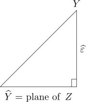
the mean vectors and Covariance matrices determined in result 1 enables us to predict sampling
properties of the least squares predictors.
SAMPLING PROPERTIES
Introduction:
We first consider the problem of estimating the mean vector were the predictor variable, us
values
\[Z_0 = \begin {bmatrix} 1 & Z_{01} & \cdots Z_{0r}\\ \end {bmatrix}' \]
then mean of \(i^{\text {th}}\) response variable is \(Z_0'B_{(i)1}\) , and this is estimated by \(\widehat {Z}_0B_{(i)1}\) the \(i^{\text {th}}\) component of the fitter
relationship. Collectively \begin {equation} \tag {11} Z_0'\widehat {B} = \begin {bmatrix} Z_0'\widehat {B}_{(i)} & \vdots & Z_0'\widehat {B}_{(2)} & \vdots & \cdots & \vdots & Z_0'\widehat {B}_{(m)}\\ \end {bmatrix}' \end {equation} is unbiased estimator of \(Z_0'\widehat {B}\)
\[E\big (Z_0'\widehat {B}_{(i)}\big ) = Z_0'E\big (\widehat {B}_{(i)}\big ) = Z_0'B_{(i)}\qquad \text {for each component}\]
Using the Covarince matrix for \(\widehat {B}_{(i)}\) and \(\widehat {B}_{(k)}\) the estimation errors \(Z'_0B_{(i)}-Z_0'\widehat {B}_{(i)}\) have covariances
\begin {align*} E\big [Z'_0\big (B_{(i)}-\widehat {B}_{(i)}\big )\big (B_{(k)}-\widehat {B}_{(k)}\big )'Z_0\big ] & = Z_0'\big (E\big (B_{(i)}-\widehat {B}_{(i)}\big )\big (B_{(k)}-\widehat {B}_{(k)}\big )'\big )Z_0\\ & = Z_0'\big (\sigma _{ik}\big (Z'Z\big )^{-1}\big )Z_0\\ & = \underbrace {\sigma _{ik}Z_0'\big (Z'Z\big )^{-1}Z_0}_{(r+1)\times (r+1)}\tag {12}\\ \end {align*}
The related problem is that of forecasting the new observation vector \(Y_0 = \begin {bmatrix} Y_{01}, & Y_{02}, & \cdots , & Y_{0m}\\ \end {bmatrix}' \) at \(Z_0\).
According to the regression model \(\, Y_{0i} = Z'_{0}B_{(i)} + \varepsilon _{oi}\,\) where the “new” error
\(\varepsilon _0 = \begin {bmatrix} \varepsilon _{01},& \varepsilon _{02}, & \cdots , \varepsilon _{0m}\\ \end {bmatrix}'\) is independent of the error \(\varepsilon \) and satisfies \(E\big (\varepsilon _{0i}\big )=0\) and \(E\big (\varepsilon _{0i},\varepsilon _{0k}\big )=\sigma _{ik}\).
The forecast error for the \(i^{\text {th}}\) component of \(Y_0\) is \begin {align*} Y_{0i} - Z'_0\widehat {B}_{(i)} & = Y_{0i} - Z_0'B_{(i)} + Z'_{0}B_{(i)} - Z_0'\widehat {B}_{(i)}\\ & = \varepsilon _{0i} - Z_0'\big (\widehat {B}_{(i)}-B_{(i)}\big ) \end {align*}
\begin {align*} \text {So}\quad E\big (Y_{0i}-Z'_0\widehat {B}_{(i)}\big ) & = E\big (\varepsilon _{0i}\big )-E\big (Z_0'\big (\widehat {B}_{(i)}-B_{(i)}\big )\big )\\ & = 0 - Z'_0 E\big (\widehat {B}_{(i)}-B_{(i)}\big )\\ & = 0- Z'_0\cdot 0\\ & = 0 \end {align*}
Indicating \(Z_0'\widehat {B}_{(i)}\) is unbiased predictor of \(Y_{0i}\).
The forecasts errors have covariances \begin {align*} E\big (Y_{0i}-Z_0'\widehat {B}_{(i)}\big )\big (Y_{0k}-Z'_0\widehat {B}_{(k)}\big ) & = E\big (\varepsilon _{0i}-Z'_0\big (\widehat {B}_{(i)}-B_{(i)}\big )\big )\big (\varepsilon _{(0k)}-Z'_0\big (\widehat {B}_{(k)}-B_{(k)}\big )\big )\\ & = E\big (\varepsilon _{0i}\varepsilon _{0k}\big ) + Z'_0E\big (\widehat {B}_{(i)}-B_{(i)}\big )\big (\widehat {B}_{(k)}-B_{(k)}\big )'Z_0-Z_0'E\big (\big (\widehat {B}_{(i)}-B_{(i)}\big )\varepsilon _{0k}\big )\\ & - E\big (\varepsilon _{0i}\big (\widehat {B}_{(k)}-B_{(k)}\big )\big )Z_0\\ & = \sigma _{ik}+Z_0'\sigma _{ik}\big (Z'Z\big )^{-1}Z_0+Z_0'\cdot 0-0\cdot Z_0\\ & = \sigma _{ik}\big (1+Z_0\big (Z'Z\big )^{-1}Z_0\big )\\ \end {align*}
Note that \(E\big (\big (\widehat {B}_{(i)}-B_{(i)}\big )\varepsilon _{0k}\big )=0\) since \(\widehat {B}_{(i)}=\big (Z'Z\big )^{-1}Z'\varepsilon _{(i)}+B_{(i)}\). is independent of \(\varepsilon _0\) future (error) while \(\varepsilon _{(i)}\) is a present error.
A similar result holds for \(E\big (\varepsilon _{0i}\big (\widehat {B}_{(k)}-B_{(k)}\big )\).
Maximum likelihood estimators and their distributions can be obtained everywhere the errors \(\varepsilon \) have
normal distribution.
Result 9.3. Let the multivariate regression model (1) hold with full rank. \(rank (Z) = r+1,\\ n\geq (r+1)+m\) and that the errors
\(\varepsilon \) have a normal distribution. Then \(\widehat {B}=\big (Z'Z\big )^{-1}Z'Y.\,\) Maximum likelihood estimator of \(B\) and \(\widehat {B}\) has a normal
distribution with \(E\big (\widehat {B}=B\big )\) and \(Cov\big (\widehat {B}_{(i)},\widehat {B}_{(k)}\big )=\sigma _{ik}\big (Z'Z\big )^{-1}\). Also \(\widehat {B}\) is independent of the maximum likelihood estimator positive
definite given by
\[\widehat {\Sigma }=\frac {\widehat {\varepsilon }'\widehat {\varepsilon }}{n}=\big (Y-Z\widehat {B}\big )\big (Y-Z\widehat {B}\big )\]
and \(\displaystyle {n\widehat {\Sigma }}\) is distributed as \(W_{n-r-1}\quad \Big (\cdot \big |\displaystyle {\Sigma }\big |\Big )\).
Proof. According to regression model, the likelihood is determined from the data \(Y= \begin {bmatrix} y_1 & y_2 & \cdots& y_n\\ \end {bmatrix}' \) whose roots are independent with \(y_i\) distributed as \(N_m\big (B'Z_j,\displaystyle {\Sigma }\big )\). We first note that \[ y-ZB = \begin {bmatrix} y_1-B'Z_1, & y_2-B'Z_2, & \cdots , & y_n-B'Z_n\\ \end {bmatrix}' \] So \(\displaystyle {\big (y-ZB\big )'\big (y-ZB\big )=\sum ^n_{j=1}\big (y_j-B'Z_j\big )\big (y_j-B'Z_j\big )'}\,\) and \begin {align*} \sum ^n_{j=1}\big (y_j-B'Z_j\big )'\Sigma ^{-1}\big (y_j-B'Z_j\big ) & = \sum ^n_{j=1}tra\Big [\big (y_j-B'Z_j\big )'\Sigma ^{-1}\big (y_j-B'Z_j\big )\Big ]\\ &= tra\Big [\Sigma ^{-1}\big (Y-ZB\big )'\big (Y-ZB\big )\Big ]\tag {1} \end {align*} □
Another preliminary calculation will enable us to express the likelihood in a simple form.
Since \(\widehat {\varepsilon }=Y-Z\hat {B}\) satisfies \(Z'\widehat {\varepsilon }=0\). Then \begin {align*} \big (Y-ZB\big )'\big (Y-ZB\big ) & = \Big [Y-Z\widehat {B}+Z\big (\widehat {B}-B\big )\Big ]\Big [Y-Z\widehat {B}+Z\big (\widehat {B}-B\big )\Big ]\\ & = \big (Y-Z\widehat {B}\big )'\big (Y-Z\widehat {B}]\big ) + \big (\widehat {B}-B\big )'ZZ'\big (\widehat {B}-B\big )\\ & = \widehat {\varepsilon }'\widehat {\varepsilon } + \big (\widehat {B}-B\big )'Z'Z\big (\widehat {B}-B\big )\tag {2} \end {align*}
Using (1) and (2) we obtain the likelihood \begin {align*} L\big (B,\Sigma \big ) & = \prod ^n_{j=1}\frac {1}{\big (2\pi \big )^{m/2}}\frac {1}{\big |\Sigma \big |^{1/2}}\exp \Big \{-\frac {1}{2}\big (y_i-B'Z_j\big )'\Sigma ^{-1}\big (y_j-B'Z_j\big )\Big \}\\ & = \frac {1}{\big (2\pi \big )^{nm/2}}\cdot \frac {1}{\big |\Sigma \big |^{n/2}}\exp \Big \{-\frac {1}{2}tra\Big [\Sigma ^{-1}\big (\widehat {\varepsilon }'\widehat {\varepsilon }+\big (\widehat {B}-B\big )'Z'Z\big (\widehat {B}-B\big )\big )\Big ]\Big \}\\ & = \frac {1}{\big (2\pi \big )^{nm/2}}\cdot \frac {1}{\big |\Sigma \big |^{n/2}}\exp \Big \{-\frac {1}{2}tra\Big (\Sigma ^{-1}\widehat {\varepsilon }'\widehat {\varepsilon }\Big )-\frac {1}{2}tra\Big [Z\big (\widehat {B}-B\big )\Sigma ^{-1}\big (\widehat {B}-B\big )'Z'\Big ]\Big \} \end {align*}
The matrix \(Z\big (\widehat {B}-B\big )\Sigma ^{-1}\big (\widehat {B}-B\big )'Z'\) is of the form \(\displaystyle {A=\Sigma ^{-\frac {1}{2}}\big (\widehat {B}-B\big )'Z'}\,\) is non-negative definite. The trace \(\displaystyle {tra\big (Z\big (\widehat {B}-B\big )\Sigma ^{-1}\big (\widehat {B}-B\big )'Z'\big )}\,\) is the sum of its eigenvalues, this trace
will equal its maximum value 0 if \(\widehat {B}=B\). This choice is unique because \(Z\) is of full rank.
Applying an earlier result with \(B=\widehat {\varepsilon }'\widehat {\varepsilon }, b=\frac {n}{2}\) and \(p=m\), we find that \(\widehat {B}\) and \(\displaystyle {\widehat {\Sigma }=\frac {\widehat {\varepsilon }'\widehat {\varepsilon }}{2}}\) are the \(MLE\) of \(B\) and \(\displaystyle {\Sigma }\), respectively , and
\begin {equation} \tag {3} L\big (\widehat {B},\widehat {\Sigma }\big ) = \frac {1}{\big (2\pi \big )^{nm/2}}\cdot \frac {n^{nm/2}}{\big |\widehat {\varepsilon }'\widehat {\varepsilon }\big |^{n/2}}e^{-nm/2}=\frac {e^{-nm/2}}{\big (2\pi \big )^{nm/2}\big |\hat {\Sigma }\big |^{n/2}} \end {equation}
It remains to establish the distribution results \(\widehat {B}_{(i)}\) and \(\widehat {\varepsilon }_{(i)}\) are linear combinations of elements of \(\varepsilon \). Specifically \begin {align*} \widehat {B}_{(i)} & = \big (Z'Z\big )^{-1}Z'\varepsilon _{(i)} + B_{(i)}\\ \widehat {\varepsilon }_{(i)} & = \big [I- Z\big (Z'Z\big )^{-1}Z'\big ]\varepsilon _{(i)}, i=1,2,\ldots ,m \end {align*}
Therefore, \(\widehat {B}_{(1)}, \widehat {B}_{(2)},\ldots ,\widehat {B}_{(m)}, \widehat {\varepsilon }_{(1)},\ldots , \widehat {\varepsilon }_{(m)}\) are jointly normal.
There mean vectors and covariances are given in equation (1) result (1).
Since \(\widehat {\varepsilon }\) and \(\widehat {B}\) have zero covariance matrix, there are independent.
Further we have the following \(I-Z\big (Z'Z\big )^{-1}Z'=\sum \limits ^{n-r-1}_{l=1}\underline {e}_l\underline {e}_l'\) where \(\underline {e}_l'\underline {e}_k=0\) for \(l\neq k\). and \(\underline {e}'_l\underline {e}_l=1\). Let \begin {align*} V_l & = \Sigma '\underline {e}_l= \begin {bmatrix} \varepsilon '_{(1)}e_l, & \varepsilon '_{2}e_l, & \cdots , & \varepsilon '_{n}e_l\\ \end {bmatrix}\\ & = e_{l_1}\varepsilon _1 + e_{l_2}\varepsilon _2 + \cdots + e_{l_n}\varepsilon _n \end {align*}
Because \(V_l, l=1,2,\ldots , n-r-1\) are linear combinations of \(\varepsilon \) , there have a joint normal distribution with \(E\big (V_l\big ) = E\big (\varepsilon '\underline {e}_l\big )\) also form our previous layout have covariance matrix \(V_l\) and \(V_k\) \[\big (e'_le_k\big ) = 0\cdot \big (\Sigma \big ) =0\qquad \text {if}\quad l\neq k\]
Consequently the independent \(l's\) are evenly distributed as \(N_m\big (0,\Sigma \big )\). Finally \begin {align*} \widehat {\varepsilon }'\widehat {\varepsilon } & = \varepsilon ' \big [I- Z\big (Z'Z\big )^{-1}Z'\big ]\varepsilon \\ & = \sum ^{n-r-1}_{\rho =1}\varepsilon 'e_le'_l\varepsilon \\ & = \sum ^{n-r-1}_{\rho =1} V_lV_l' \end {align*}
Whishart distribution \(W_{n-r-1}\Big (\cdot , \Sigma \Big )\equiv W_m\Big (n-r-1,\Sigma \Big )\)
INFERENCE
Likelihood Ratio Tests for Regression Parameters.
In multiple response analog of univariate response model the hypothesis that the responses do not
dependent on \(Z_{q+1}, Z_{q+2}, \ldots , Z_r\) becomes \(H_0: B_{(2)} =B = 0\) where
\(B = \begin {bmatrix} B_{(1)_{(q\times 1)\times m}}\\ \cdots \\ B_{2_{(l-q)\times m}}\\ \end {bmatrix}\) setting \(Z= \begin {bmatrix} Z_1 & \vdots & Z_2\\ n\times (q+1) & \vdots & n\times (n-q)\\ \end {bmatrix}\) the general model becomes
\[E(Y)= \begin {bmatrix} Z_1 & \vdots & Z_2\\ \end {bmatrix} \begin {bmatrix} B_{(1)}\\ \cdots \\ B_{(2)}\\ \end {bmatrix} =Z_1B_{(1)} + Z_2B_{(2)}\]
Under \(H_0: B_{(2)} = 0\)
\(Y= Z_1B_{(1)} + \varepsilon \) and the likelihood ratio test of \(H_0\) is based on the quantities involved in the extra sum of squares and
cross-products
\[\big (Y-Z_1\widehat {B}_{(1)}\big )'\big (Y-Z_1\widehat {B}_{(1)}\big ) - \big (Y-Z\widehat {B}\big )'\big (Y-Z\widehat {B}\big )=n\big (\widehat {\Sigma }_1-\widehat {\Sigma }\big )\]
where \(\widehat {B}_{(1)}=\big (Z_1'Z_1\big )^{-1}Z'_1Y\) and \(\sum \limits ^n_l=\big (Y-Z_l\widehat {B}_{(l)}\big )'\big (Y-Z_l\widehat {B}_{(l)}\big )/n\).
The likelihood ratio can be expressed of generalised variances so
\begin {align*} \Delta & = \frac {\max \limits _{B_{(i)},\Sigma }L\big (B_{(i)},\Sigma \big )}{\max \limits _{B,\Sigma }L\big (B,\Sigma \big )} = \frac {L\Big (\widehat {B}_{(i)},\widehat {\Sigma }_{(i)}\Big )}{L\Big (\widehat {B},\widehat {\Sigma }\Big )}\\\\ & = \Bigg (\frac {\big |\widehat {\Sigma }\big |}{\big |\widehat {\Sigma }_l\big |}\Bigg )^{\frac {n}{2}} \end {align*}
equivalent Wilk’s Lambda statistic \(\Delta ^{2/n}=\frac {\big |\widehat {\Sigma }\big |}{\big |\widehat {\Sigma }_l\big |}\) can be used.
Result 9.4. Let the multivariate multi regression model (1) hold with \(Z\) of full rank \(r+1\) and \((r+1)+m<n\). Let
the error \(\varepsilon \) be normally distributed under \(H_0: B_{(2)} =0\).
\(n\widehat {\Sigma }\thicksim W_m\big (n-r-1, \Sigma \big )\) independent of \(n\big (\widehat {\Sigma }_l-\widehat {\Sigma }\big )\) which in turn \(n\big (\widehat {\Sigma }_l-\widehat {\Sigma }\big )\thicksim W_m\big (r-q,\Sigma \big )\).
The likelihood ratio test of \(H_0\) is equivalent to rejection \(H_0\) for large values of \begin {align*} -2\ln \Delta & = -n\ln \Bigg (\frac {\big |\widehat {\Sigma }\big |}{\big |\widehat {\Sigma }_l\big |}\Bigg )\\\ & = -n\ln \frac {n\widehat {\Sigma }}{\Big |n\widehat {\Sigma }+n\big (\widehat {\Sigma }_l-\widehat {\Sigma }\big )\Big |} \end {align*}
for large \(n\) the modified statistic is \[-\big [n-r-1-\frac {1}{2}(m-r+q+1)\big ]\ln \Bigg (\frac {\big |\widehat {\Sigma }\big |}{\big |\widehat {\Sigma }_l}\Bigg )\]
has a close to approximation a Chi-square distribution. i.e \(\thicksim \chi ^2_{m(r-q)}\).
Example 9.5. The services in three locations of a large restaurant chain was rated according
to the majors by male and female patrons.
Suppose we consider a regression under that allows for the effects and the location gender interrelation
services quality indexes.
A computer program provides the following
\[\begin {pmatrix} \text {Residual sum of}\\ \text {squares and cross}\\ \text {-products}\\ \end {pmatrix}= n\widehat {\Sigma }= \begin {pmatrix} 2977.39 & 1021.72\\ 1021.72 & 2050.95\\ \end {pmatrix}\]
\[\begin {pmatrix} \text {Extra sum of }\\ \text {squares and }\\ \text {cross-products}\\ \end {pmatrix}=n\big (\widehat {\Sigma }-\Sigma \big )= \begin {pmatrix} 441.76 & 246.16\\ 246.16 & 364.12\\ \end {pmatrix}\]
Let \(B_2\) be the matrix of interrelationships presentation for the two responses although the sample size \(n=18\) is not large we shall illustrate the calculation involved in the test of \(B_{(2)} = 0 \) setting \(\alpha = 0.05\) we set \(H_0\) by referring \begin {align*} &-\big [n-r_1-1-\frac {1}{2}(m-r_1+q_1+1)\big ]\times \ln \frac {\big |n\widehat {\Sigma }\big |}{\Big |n\widehat {\Sigma }+n\big (\widehat {\Sigma }_l-\widehat {\Sigma }\big )\Big |}\\\\ & = -\big [18 - 5 -1 -\frac {1}{2}(2-5+3+1)\big ]\ln (0.7605)\\ & = 3.28\qquad \text {to a Chi-square} \end {align*}
\[n(r_1-q_1)=2(2) = 4 df\]
Since \(3.28 < \chi ^2_{4,(0.05)}= 9.49\), we fail to reject \(H_0\)
Interrelation term not needed.
Other Tests
Tests other than the likelihood ratio have been proposed for the multivariate multiple model. The most prominent alternative is the Roy’s greatest Root which rejects \(H_0:_{\eta }B_{(2)}=\underline {0}\) for where \(\eta \) is the greater root of \[\Bigg |\Big (\widehat {\Sigma }_l-\widehat {\Sigma }\Big )-\eta \widehat {\Sigma }\Bigg | = 0\qquad \text {Polynomial of order }m\] tables of critical values are available for quantities \(\displaystyle {U=\frac {\eta }{1 + \eta }}\,\) critical value of \(\eta _{\alpha }\) are given \[\eta _{\alpha } = \frac {\theta _{\alpha }}{1- \theta _{\alpha }}\]
Hotellings-Lawley Trace test is based on the the sum of the roots \(\eta \).
Wilk’s Lambda, Roy’s Greatest Root and Hotelling - Lawley are nearly equivalent for large sample
sizes.
Predictions for Multivariate Multiple Regression
Suppose the model \(Y= ZB + \varepsilon \) with normal errors \(\varepsilon \) has been fitted and checked for any inadequacies.
If the model is adequate it can be employed for predication purpose.
One problem is to predict the mean responses corresponding to fixed \(Z_0\).
Inference about the mean response can be made using the distribution theory using result
2.
From this result we determine \(\widehat {B}'Z_0\) is distributed as \(N_m\big (B'Z_0,Z_0'\big (Z'Z\big )^{-1}Z_0\Sigma \big )\) and \(n\widehat {\Sigma }\) is independently distributed as \(W_m\big (n-r-1,\Sigma \big )\).
Then unknown value of the regression function at \(Z_0\) is \(B'Z_0\) so from the discussion of the Hotellings - \(T^2\) we write \begin {equation} \tag {4} T^2 = \Bigg (\frac {\widehat {B}'Z_0-B'Z_0}{\sqrt {\Big (Z'_0\big (Z'Z\big )^{-1}Z_0\Big )}}\Bigg )'\Bigg (\frac {n\widehat {\Sigma }}{n-r-1}\Bigg )^{-1} \Bigg (\frac {\widehat {B}'Z_0-B'Z_0}{\sqrt {Z_0'\big (Z'Z\big )^{-1}Z_0}}\Bigg ) \end {equation} and the \(100(1-\alpha )\%\) confidence ellipsoid for \(B'Z_0\) is provided by the inequality
\begin {align*} \big (B'Z_0-\widehat {B}'Z_0\big )'\Bigg (\frac {n\widehat {\Sigma }}{n-r-1}\Bigg )^{-1}\big (B'Z_0-\widehat {B}'Z_0\big ) \leq Z_0'\big (Z'Z\big )^{-1}Z_0\Bigg [\Bigg (\frac {m(n-r-1)}{n-r-m}\Bigg )F_{m,n-r-m}(\alpha )\Bigg ] \end {align*}
where \(F_{m,n-r-m}(\alpha )\) is the upper \((100 \alpha ^{\text {th}})\) percentile of an \(F-\) distribution with \(m\) and \(n-r-m\) \(df\).
The \(100(1-\alpha )\%\) simultaneous confidence intervals for \(E(Y_i) = Z_0'B_{(i)}\)
\begin {align*} Z_0'\widehat {B}_{(i)} & \pm \sqrt {\Bigg (\frac {m(n-r-1)}{n-r-m}\Bigg )F_{m,n-r-m}(\alpha )}\times \sqrt {Z_0'\big (Z'Z\big )^{-1}Z_0\Bigg (\frac {n}{n-r-1}\Bigg )\widehat {\sigma }_{ii}} \end {align*}
where \(\widehat {B}_{(i)}\) is the \(i^{\text {th}}\) column of \(\widehat {B}\) and \(\widehat {\sigma }_{ii}\) is the \(i^{\text {th}}\) diagonal element of \(\widehat {\Sigma }\).
Questions on this section
Stuck on something here? Ask below and it stays attached to this topic.