8.1 Incorporating Data
A vector of observations may be decomposed as follows:
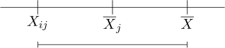
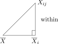
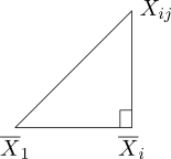
\begin {equation} \tag {4} X_{ij}-\overline {X} = \overline {X}_i-\overline {X} + \big (X_{ij} - \overline {X}_i\big ) \end {equation} where
- \(\underline {X}_{ij}=\) observation
- \(\overline {\underline {X}}=\) overall sample mean, \(\underline {\hat {\mu }}\)
- \(\overline {X}_i- \overline {X} = \) Estimate of treatment effect \(\tau _i\)
- \(X_{ij} -\overline {X}_i =\) Residual estimate of error, \(\hat {e}_{ij}\)
The decomposition (4) leads to the univariate analog of univariates sum of squares break up specifically (1) the left hand side becomes \[\sum ^g_{i=1}\sum ^{n_i}_{j=1}\big (\underline {X}_{ij}-\underline {\overline {X}}\big )\big (\underline {X}_{ij}-\overline {\underline {X}}\big )'\]
as the total corrected sum of squares and cross products
\begin {equation} \tag {5} 2.1\qquad \sum ^g_{i}n_i\big (\overline {\underline {X}}_i-\overline {\underline {X}}\big )\big (\overline {\underline {X}}_i-\overline {\underline {X}}\big )' \end {equation} As the Between treatments sum of squares and cross products
\begin {equation} \tag {6} 2.2\qquad \sum ^g_{i=1}\sum ^{n_i}_{j=1}\big (\underline {X}_{ij}-\overline {\underline {X}}_i\big )\big (\underline {X}_{ij}-\overline {\underline {X}}_i\big )' \end {equation}
As the residual within sum of squares and cross products.
2.2 can also be expressed as follows \begin {align*} \textbf {W} & = \sum ^g_{i=1}\sum ^{n_i}_{j=1}\big (\underline {X}_{ij}-\overline {\underline {X}}_i\big )\big (\underline {X}_{ij}-\overline {\underline {X}}_i\big )'\\ & = \sum ^g_{i=1}(n_i-1)S_i\\ & = (n_1-1)S_1 + (n_2-1)S_2 + \cdots + (n_g-1)S_g\tag {7} \end {align*}
The matrix generalisation, where \(S_i\) is the sample covariance matrix for the \(i^{\text {th}}\) sample group.
\((n_1+n_2-2)S\) pooled matrix encountered in the two sample situation.
To test the hypothesis of no treatment effect. \[H_0: \underline {\tau _1} = \underline {\tau _2} = \cdots = \underline {\tau _g}=\underline {0} \qquad \text {or}\quad H_0: \underline {\mu _1} = \underline {\mu _2}=\cdots = \underline {\mu _g}\]
\begin {align*} \underline {\mu }_1 & = \underline {\mu } + \underline {\tau }_1\\ \underline {\mu }_2 & = \underline {\mu } + \underline {\tau }_2\\ \vdots & \\ \underline {\mu }_g & = \underline {\mu } + \underline {\tau }_g\\\\ \sum \underline {\mu }_i & = g\underline {\mu } + \sum \underline {\tau }_i \end {align*}
We utilise the relative sizes of the residual and total (corrected sum of squares and cross products matrix terms). The results are often summarised in the table known as the MANOVA
| Source of | Matrix of \(SS\) | Degrees of |
| Variation | and Cross Products | Freedom \((df)\) |
| Treatment | \(\textbf {B}=\displaystyle {\sum ^g_{i=1}n_i\big (\overline {\underline {X}}_i-\overline {\underline {X}}\big )\big (\overline {\underline {X}}_i-\overline {\underline {X}}\big )'}\) | \(g-1\) |
| Residual (Error) | \(\textbf {W}=\displaystyle {\sum ^g_{i=1}\sum ^{n_i}_{j=1}\big (\underline {X}_{ij}-\overline {\underline {X}_i}\big )\big (\underline {X}_{ij}-\overline {\underline {X}_i}\big )'}\) | \(\displaystyle {\sum ^g_{i=1}n_i-g}\) |
| Total (corrected) | \(\textbf {B}+ \textbf {W}=\displaystyle {\sum ^g_{i=1}\sum ^{n_i}_{j=1}\big (\underline {X}_{ij}-\overline {\underline {X}}\big )\big (\underline {X}_{ij}-\overline {\underline {X}}\big )'}\) | \(\displaystyle {\sum ^g_{i=1}n_i-1}\) |
| For the Mean | ||
\[X_{ij} = \mu + \tau _i + e_{ij} \thicksim N_p\big (\underline {0},\Sigma \big )\qquad \text {estimates}\quad X_{ij}=\underline {\overline {X}}+\overline {\underline {X_i}}\cdot \overline {\underline {X}} + X_{ij}-\overline {\underline {X}_i}\]
The degrees of freedom correspond to the univariate geometric and also to multivariate distribution
theory of the Wishart densities.
The test of \(H_0: \underline {\tau }_1 = \underline {\tau }_2 = \cdots = \underline {\tau }_g = \underline {0}\) utilise the Wilk’s Lambda \begin {align*} \Delta _W & = \frac {\Big |\textbf {W}\Big |}{\Big |\textbf {B}+\textbf {W}\Big |}\\\\ & = \frac {\Bigg |\displaystyle {\sum ^g_{i=1}\sum ^{n_i}_{j=1}\big (\underline {X}_{ij}-\overline {\underline {X}_i}\big )\big (\underline {X}_{ij}-\overline {\underline {X}_i}\big )'}\Bigg |}{\Bigg |\displaystyle {\sum ^g_{i=1}\sum ^{n_i}_{j=1}\big (\underline {X}_{ij}-\overline {\underline {X}}\big )\big (\underline {X}_{ij}-\overline {\underline {X}}\big )'}\Bigg |}\tag {9} \end {align*}
There are various cases of which \(\Delta \) leads to exact distributions.
| No. of | No. of | |
| variables | groups | Sampling distributions for multivariate normal data |
| \(P=1\) | \(g\geq 2\) | \(\Bigg (\frac {\sum n_i-g}{g-1}\Bigg )\Bigg (\frac {1-\Delta }{\Delta }\Bigg )\thicksim F_{g-1,\sum n_i-g}\) |
| \(p=2\) | \(g\geq 2\) | \(\Bigg (\frac {\sum n_i-g-1}{g-1}\Bigg )\Bigg (\frac {1-\sqrt {\Delta }}{\sqrt {\Delta }}\Bigg )\thicksim F_{2(g-1),2(\sum n_i-g-1)}\) |
| \(p\geq 1\) | \(g=2\) | \(\Bigg (\frac {\sum n_i-p-1}{p}\Bigg )\Bigg (\frac {1-\Delta }{\Delta }\Bigg )\thicksim F_{p,\sum n_i-p-1}\) |
| \(p\geq 1\) | \(g=2\) | \(\Bigg (\frac {\sum n_i - p -2}{p}\Bigg )\Bigg (\frac {1-\sqrt {\Delta }}{\sqrt {\Delta }}\Bigg )\thicksim F_{2p,2(\sum n_i-p-2)}\) |
\begin {align*} & Pr\big (\ln \Delta ^* < \ln \Delta ^*_c = \Delta '_c\big )\\ & Pr\Big (-\big (n-1-\frac {p+g}{2}\big )\ln \Delta ^* < \Delta '_c\Big )\\ & Pr\Big (\chi ^2_{p(g-1)}\leq \Delta _c\Big )= \alpha \\ \end {align*}
Example 8.1. Suppose that an experiment was performed in which 4 groups of students were
sent to interview holds on certain issues. For correctness, suppose that there were \(n=3\) students per
group and 2 questions were asked on each house hold the expenses on the house hold in previous
months in each month recorded separate. The data imaginary are recorded in the following
table in 100’s of kwacha.
| measurements (100’s of Kwacha)
| |||
| Group | Student | Month 1 | Month 2 |
| 1 | 4 | 6 | |
| 1 | 2 | 2 | 5 |
| 3 | 3 | 4 | |
| 1 | 4 | 5 | |
| 2 | 2 | 5 | 4 |
| 3 | 6 | 6 | |
| 1 | 6 | 6 | |
| 3 | 2 | 7 | 8 |
| 3 | 8 | 7 | |
| 1 | 7 | 6 | |
| 4 | 2 | 9 | 8 |
| 3 | 8 | 7 | |
Test for the difference in mean vector in the four groups. \[H_0: \underline {\mu }_1 = \underline {\mu }_2=\underline {\mu }_3=\underline {\mu }_4\]
Solution. \[X_{ij} \thicksim N_2\big (\underline {\mu }_i,\Sigma \big ), i=1,2,3,4\]
\[\overline {X}=\begin {pmatrix} \overline {X}_1\\ \overline {X}_2\\ \end {pmatrix}= \begin {pmatrix} \sum X_{1j}/12\\ \sum X_{2j}/12\\ \end {pmatrix}= \begin {pmatrix} 5.75\\ 6\\ \end {pmatrix} \]
\[n_1=3;\quad \overline {X}_1=\begin {pmatrix} (4+2+3)/3\\ (6+5+4)/3\\ \end {pmatrix}= \begin {pmatrix} 3\\ 5\\ \end {pmatrix} \]
\[n_2=3;\quad \overline {X}_2= \begin {pmatrix} 5\\ 5\\ \end {pmatrix} \]
\[\overline {X}_3= \begin {pmatrix} 7\\7\\ \end {pmatrix} \qquad \overline {X}_4= \begin {pmatrix} 8\\ 7\\ \end {pmatrix} \]
\begin {align*} \textbf {B} & = \sum ^g_in_i\big (\overline {\underline {X}_i}-\overline {\underline {X}}\big )\big (\overline {\underline {X}_i}-\overline {\underline {X}}\big )'\\ & = \sum ^4_1 3\big (\overline {\underline {X}_i}-\overline {\underline {X}}\big )\big (\overline {\underline {X}_i}-\overline {\underline {X}}\big )'\\ & = 3\begin {pmatrix} -2.75\\ -1\\ \end {pmatrix} \begin {pmatrix} -2.75 & -1\\ \end {pmatrix} + 3\begin {pmatrix} -0.75\\ 1\\ \end {pmatrix} \begin {pmatrix} -0.75 & 1\\ \end {pmatrix}\\ & + 3 \begin {pmatrix} 1.25\\1\\ \end {pmatrix} \begin {pmatrix} 1.25 & 1\\ \end {pmatrix} + 3\begin {pmatrix} 2.25\\ 1\\ \end {pmatrix} \begin {pmatrix} 2.25 & 1\\ \end {pmatrix}\\\\ \implies \quad \textbf {B}& = \begin {pmatrix} 44.25 & 21\\ 21 & 12.00\\ \end {pmatrix}\\\\ \end {align*}
\[ \textbf {W}= \sum ^4_{i=1}\sum ^3_{j=1}\big (\underline {X}_{ij}-\overline {X}_i\big )\big (\underline {X}_{ij}-\overline {X}_i\big )'\]
\begin {align*} G_1: & \begin {pmatrix} 1\\ 1\\ \end {pmatrix} \begin {pmatrix} 1, & 1\\ \end {pmatrix} + \begin {pmatrix} -1\\ 0\\ \end {pmatrix} \begin {pmatrix} -1, & 0\\ \end {pmatrix} + \begin {pmatrix} 0\\ -1\\ \end {pmatrix} \begin {pmatrix} 0, & -1\\ \end {pmatrix}\\\\ & = \begin {pmatrix} 1 & 1\\ 1 & 1\\ \end {pmatrix} + \begin {pmatrix} 1 & 0\\ 0 & 0\\ \end {pmatrix} + \begin {pmatrix} 0 & 0\\ 0 & 1\\ \end {pmatrix}\\\\ & = \begin {pmatrix} 2 & 1\\ 1 & 2\\ \end {pmatrix}\\ \end {align*}
\begin {align*} G_2: & \begin {pmatrix} -1\\0\\ \end {pmatrix} \begin {pmatrix} -1, & 0\\ \end {pmatrix} + \begin {pmatrix} 0\\ -1\\ \end {pmatrix} \begin {pmatrix} 0, & -1\\ \end {pmatrix} + \begin {pmatrix} 1\\1\\ \end {pmatrix} \begin {pmatrix} 1, & 1\\ \end {pmatrix}\\\\ & =\begin {pmatrix} 1 & 0\\ 0 & 0\\ \end {pmatrix} + \begin {pmatrix} 0 & 0\\ 0 & 1\\ \end {pmatrix} + \begin {pmatrix} 1 & 1\\ 1 & 1\\ \end {pmatrix}\\\\ & = \begin {pmatrix} 2 & 1\\ 1 & 2\\ \end {pmatrix}\\ \end {align*}
\begin {align*} G_3: & \begin {pmatrix} -1\\-1\\ \end {pmatrix} \begin {pmatrix} -1, & -1\\ \end {pmatrix} + \begin {pmatrix} 0\\ 1\\ \end {pmatrix} \begin {pmatrix} 0, & 1\\ \end {pmatrix} + \begin {pmatrix} 1\\0\\ \end {pmatrix} \begin {pmatrix} 1, & 0\\ \end {pmatrix}\\\\ & = \begin {pmatrix} 1 & 1\\ 1 & 1\\ \end {pmatrix} + \begin {pmatrix} 0 & 0\\ 0 & 1\\ \end {pmatrix} + \begin {pmatrix} 1 & 0\\ 0 & 0\\ \end {pmatrix}\\ & = \begin {pmatrix} 2 & 1\\ 1 & 2\\ \end {pmatrix}\\ \end {align*}
\begin {align*} G_4: & \begin {pmatrix} -1\\ -1\\ \end {pmatrix} \begin {pmatrix} -1, & -1\\ \end {pmatrix} + \begin {pmatrix} 1\\ 1\\ \end {pmatrix} \begin {pmatrix} 1, & 1\\ \end {pmatrix} + \begin {pmatrix} 0 \\ 0\\ \end {pmatrix} \begin {pmatrix} 0, & 0\\ \end {pmatrix}\\\\ & = \begin {pmatrix} 1 & 1\\ 1 & 1\\ \end {pmatrix} + \begin {pmatrix} 1 & 1\\ 1 & 1\\ \end {pmatrix} + \begin {pmatrix} 0 & 0\\ 0 & 0\ \end {pmatrix}\\\\ & = \begin {pmatrix} 2 & 2\\ 2 & 2\\ \end {pmatrix}\\ \end {align*}
\begin {align*} \implies \quad \textbf {W} & = G_1 + G_2 + G_3 + G_4\\ & = \begin {pmatrix} 2 & 1\\ 1 & 2\\ \end {pmatrix} + \begin {pmatrix} 2 & 1\\ 1 & 2\\ \end {pmatrix} + \begin {pmatrix} 2 & 1\\ 1 & 2\\ \end {pmatrix} +\begin {pmatrix} 2 & 2\\ 2 & 2\\ \end {pmatrix}\\\\ \textbf {W} & = \begin {pmatrix} 8 & 5\\ 5 & 8\\ \end {pmatrix}\\\\ \end {align*}
Wilks’ Lambda \(\Delta \) statistic is \begin {align*} \Delta & = \frac {\Big |\textbf {W}\Big |}{\Big |\textbf {B}+\textbf {W}\Big |} = \frac { \begin {vmatrix} 8 & 5\\ 5 & 8\\ \end {vmatrix} }{ \begin {vmatrix} 52.25 & 26\\ 26 & 20\\ \end {vmatrix} }\\\\ & = \frac {64-25}{1045-676}=\frac {39}{369}\\\\ & = 0.106\\ \end {align*}
\[p=2, g\geq 2\qquad \Bigg (\frac {\sum n_i-g-1}{g-1}\Bigg )\Bigg (\frac {1-\sqrt {\Delta }}{\sqrt {\Delta }}\Bigg )\thicksim F_{2,(g-1)}\]
\[\implies \quad g=4, 2(g-1)=2(3)=6\]
\[2\big (\sum n_i -g-1\big ) = 2 (12-4-1) =14\]
\[F_{6,14,0.95}=2.85\]
\[F_{obse} = \Bigg (\frac {12-5}{3}\Bigg )\Bigg (\frac {1-\sqrt {0.10569}}{\sqrt {0.10569}}\Bigg )=4.8439\]
Since \(F_{obse} = 4.84>2.85\) we reject \(H_0\) and conclude the average means of expenditure are different for the four
groups.
Questions on this section
Stuck on something here? Ask below and it stays attached to this topic.