5.6 Confidence Regions

1.

Here we extended the concept of the unvariate confidence interval to a multivariate confidence region.

2.

The region is determined by the data and for the moment, denotes it by \(R(X)\), where \(X= \begin {pmatrix} \underline {X}_1,\underline {X}_2,\ldots ,\underline {X}_n\\ \end {pmatrix}\)is the data matrix.

3.

The region \(R(X)\) is said to the \(100(1-\alpha )\%\) confidence region if before the sample is selected.

\(Pr( R(X)\) will cover the true \(\underline {\theta })=1-\alpha \qquad (1)\)

4.

This \(Pr\) is calculated under the true but unknown value of \(\theta \).

5.

The confidence region for \(\underline {\mu }\) of \(P-\) dimensional normal population from our previous work satisfies. \begin {equation} \tag {2} Pr\Bigg [n\big (\overline {\underline {X}}-\underline {\mu }\big )'S^{-1}\big (\overline {\underline {X}}-\underline {\mu }\big )\leq \frac {(n-1)p}{n-p}F_{p,n-p}(\alpha )\Bigg ] = 1 - \alpha \end {equation}

6.

For a particular sample \(\overline {\underline {X}}\) and \(S\) can be computed and the inequality \[ n\big (\overline {\underline {X}}-\underline {\mu }\big )'S^{-1}\big (\overline {\underline {X}}-\underline {\mu }\big )\leq \frac {(n-1)p}{n-p}F_{p,n-p}(\alpha )\] will define a region \(R(X)\) and this particular region is an ellipsoid centred at \(\overline {\underline {X}}\).

Beginning at the centre \(\overline {\underline {X}}\) the axes of the confidence ellipsoid are \[\pm \sqrt {\lambda _i}\sqrt {\frac {p(n-1)}{n(n-p)}F_{p,n-p,(1-\alpha )}}\underline {e}_i\] where \(S\underline {e}_i = \lambda _i\underline {e}_ip, i= (1)p\).

Simultaneous Confidence Statements

The confidence region in (3) \(\displaystyle { n\big (\overline {\underline {X}}-\underline {\mu }\big )'S^{-1}\big (\overline {\underline {X}}-\underline {\mu }\big ) \leq C^2}\,\) where \(C\) is constant. Correctly asses the joint knowledge concern values for \(\underline {\mu }\). There is need, however to make statements about the individual components means or specific linear combinations.

Let \(\underline {X}\thicksim N_p\big (\underline {\mu },\Sigma \big )\) and consider the linear combinations. \begin {equation} \tag {4} Z = L_1X_1 + L_2X_2 + \cdots + L_pX_p \end {equation} From the previous work, we know that \begin {equation} \tag {5} \mu _Z =E(Z) = E\big (\underline {L}'\underline {X}\big ) = \underline {L}'E(\underline {X})=L'\underline {\mu } \end {equation} and \(\, \displaystyle {var(Z) = var\big (\underline {L}'\underline {X}\big ) = \underline {L}'var(\underline {X})\underline {L}=\underline {L}'\Sigma \underline {L}\qquad (6)}\)

Since \(Z\) is a linear combination of normal variance, \(Z\) itself has a normal distribution. \begin {equation} \tag {7} Z\thicksim N\big (\underline {L}'\underline {\mu }, \underline {L}'\Sigma \underline {L}\big ) \end {equation}

Once sample values are available, we can estimate \(\mu _Z= \underline {L}'\underline {\mu }\) and \(\Sigma _Z = \underline {L}'\Sigma \underline {L}\) in that case sample estimate become \begin {equation} \tag {8} \overline {Z} = \underline {L}'\overline {\underline {X}} \end {equation} \(S^2_2 = \displaystyle {\underline {L}'S\underline {L}}\), where \(S\) is the usual sample covariance matrix.

For the fixed \(L\), and \(\sigma ^2_Z\) unknown a \(100(1-\alpha )\%\) confidence interval for \(\mu _Z = \underline {L}'\underline {\mu }\) based on student’s \(t\) ratio \begin {equation} \tag {9} t = \frac {\overline {Z}-\mu _Z}{S_Z/\sqrt {n}}=\frac {\sqrt {n}\big (\underline {L}'\overline {\underline {X}}-\underline {L}'\underline {\mu }\big )}{\sqrt {\underline {L}'S\underline {L}}} \end {equation} and leads to the statement \(M.E=\) Margin of Error

\[\overline {Z}-t_{n-1,(1-\alpha /2)}\cdot \frac {S_Z}{\sqrt {n}}\leq \mu _Z \leq \overline {Z}+t_{n-1,(1-\alpha /2}\cdot \frac {S_Z}{\sqrt {n}}\]

or

\begin {equation} \tag {10} \underline {L}'\overline {\underline {X}}-t_{n-1, (1-\alpha /2)} \sqrt {\frac {\underline {L}'S\underline {L}}{n}} \leq L'\mu \leq \underline {L}'\overline {\underline {X}} + t_{n-1,(1-\alpha /2)}\frac {\sqrt {\underline {L}'S\underline {L}'}}{\sqrt {n}} \end {equation}

It can be shown that \(T^2=n\big (\overline {\underline {X}}-\underline {\mu }\big )'S^{-1}\big (\overline {\underline {X}}-\underline {\mu }\big )\leq C^2\) implies that \(\frac {n\big (L'\overline {\underline {X}}-L'\underline {\mu }\big )^2}{L'SL}\leq C^2\quad \forall L\) or \[L'\overline {\underline {X}}-C\sqrt {\frac {L'SL}{n}}\leq \underline {L}'\underline {\mu }\leq L'\underline {\overline {X}}+C\sqrt {\frac {L'SL}{n}}\quad \cdots \quad (*)\]

and choosing \(C^2= \frac {p(n-1)}{n-p}F_{p,n-p}(1-\alpha )\), then the interval \begin {equation} \tag {11} L'\overline {\underline {X}}- \sqrt {\frac {p(n-1)}{n-p}F_{p,n-p,(1-\alpha )}\frac {L'SL}{n}}\leq \underline {L}'\underline {\mu }\leq L'\overline {\underline {X}}+\sqrt {\frac {p(n-1)}{n-p}F_{p,n-p,(1-\alpha )}\frac {L'SL}{n}} \end {equation} a \(100(1-\alpha )\%\) interval in (11) may be refereed as \(T\) interval since coverage probability for various choices may be determined by the Hotelling’s \(T^2\) distribution associated with \(F\) distribution.

Various choices of \(L\) lead to intervals of individual component means \begin {align*} L'_1 & = \begin {pmatrix} 1, & 0, & 0, & \cdots & 0\\ \end {pmatrix}\\ L'_2 & = \begin {pmatrix} 0, & 1, & 0, & \cdots & 0\\ \end {pmatrix}\\ \vdots & \\ L'_p & = \begin {pmatrix} 0, & 0, & 0, & \cdots & 1\\ \end {pmatrix}\\ \end {align*}

\begin {align*} L_1 & : \overline {X}_1-\sqrt {\frac {p(n-1)}{n-p}F_{p,n-p,1-\alpha }\frac {S_{11}}{n}}\leq \mu _1\leq \overline {X}_1+ \sqrt {\frac {p(n-1)}{n-p}F_{p,n-p,1-\alpha }\frac {S_{11}}{n}}\\\\ L_2 & : \overline {X}_2-\sqrt {\frac {p(n-1)}{n-p}F_{p,n-p,1-\alpha }\frac {S_{22}}{n}}\leq \mu _2\leq \overline {X}_2+ \sqrt {\frac {p(n-1)}{n-p}F_{p,n-p,1-\alpha }\frac {S_{22}}{n}}\\ & \vdots \\ & \vdots \\ L_p & : \overline {X}_p-\sqrt {\frac {p(n-1)}{n-p}F_{p,n-p,1-\alpha }\frac {S_{pp}}{n}}\leq \mu _2\leq \overline {X}_2+ \sqrt {\frac {p(n-1)}{n-p}F_{p,n-p,1-\alpha }\frac {S_{pp}}{n}}\\ \end {align*}

Data
\(X_1=\) score out of 100 in assignment 1
\(X_2=\) score out of 100 in assignment 2
\(X_3=\) score out of 100 in assignment 3

This is an example of a repeated measurements design in which each has three measurements.

Let \(\underline {\mu }=\begin {pmatrix} \mu _1, & \mu _2, & \mu _3\\ \end {pmatrix}'\) and assume that \(\underline {X}_i\thicksim N_3\big (\underline {\mu },\Sigma \big )\) where \(\underline {X}_i\) is a vector of scores for the \(i^{\text {th}}\) student

1.

Test \(H_0:\mu _1 = \mu _2 = \mu _2\) vs \(H_a: \mu _i\neq \mu _j\) for some \(i\neq j\).

2.

Find a \(95\%\) confidence region for the true mean vector \(\underline {\mu }=\begin {pmatrix} \mu _1\\ \mu _2\\ \mu _3\\ \end {pmatrix} \)

3.

Find a \(95\%\) confidence interval for \(\mu = \frac {1}{3}\big (\mu _1+\mu _2+\mu _3\big )\).

4.

Find a \(95\%\) C.I for \(\mu _1\), \(\mu _2\) and \(\mu _3\) respectively.

5.

Determine whether \(\mu _0 = \begin {pmatrix} 50, & 50, & 50\\ \end {pmatrix}\).

\[S^{-1} = \begin {pmatrix} 0.0183304 & & \\ 0.02359 & 0.0024021 & \\ 0.0015441 & 0.0004656 & 0.0069898\\ \end {pmatrix}\]

\[n=36, t=p=3\]

1.

\(-\)

\(H_0: \mu _1 = \mu _2 = \mu _3\) vs \(H_a: \mu _i \neq \mu _j\) for some \(i\neq j\).

\(-\)

Test \[T^2=n\big (C\overline {X}\big )'\big (CSC'\big )^{-1}\big (C\overline {X}\big )\]

\[C=\begin {pmatrix} 1 & -1 & 0\\ 0 & 1 & -1\\ \end {pmatrix}\]

\(-\)

Decision:
Reject \(H_0\) if \(F_{obs}>F_{2,34,0.95}=3.275\)

\(-\)

Conclusion: \[T^2 = 11.657772\]

\begin {align*} F_{obs} & = \frac {n-C}{(n-1)C}T^2\qquad C- \text {number of rows in the matrix } C\\ & = \frac {36-2}{(36-1)2}(11.657772)\\ & = 5.662 \end {align*}

Since \(F_{obs} > 3.275\) we reject \(H_0\) and conclude that the 3 means are not equal. In other terms the average performance in the three assignments are different.

Problem 5.1. verify \(T^2\)

2.

The \(95\%\) confidence region is give by \[ n\big (\overline {X}-\underline {\mu }\big )'S^{-1}\big (\overline {X}-\underline {\mu }\big ) \leq \frac {p(n-1)}{n-p}F_{p,n-p}(1-\alpha )\]

\begin {align*} F_{3,36-3}(0.95) & = F_{3,33}(0.95)\\ & = \frac {1}{2}(2.92+2.84)\\ & = 2.88\\ \end {align*}

\[\frac {p(n-1)}{n-p}F_{3,33}(0.95) = \frac {3\times 35}{33}\times 2.88= 9.164\]

\[\overline {\underline {X}}-\underline {\mu } = \begin {pmatrix} 76.44 - \mu _1\\ 69.75 - \mu _2\\ 68.06 - \mu _3\\ \end {pmatrix} \]

\[36 \begin {pmatrix} 76.44 - \mu _1\\ 69.75 - \mu _2\\ 68.06 - \mu _3\\ \end {pmatrix}' \begin {pmatrix} 0.0183304 & & \\ 0.0002359 & 0.002401 & \\ 0.0015441 & 0.004646 & 0.06989\\ \end {pmatrix} \begin {pmatrix} 76.44 - \mu _1\\ 69.75 - \mu _2\\ 68.06 - \mu _3\\ \end {pmatrix} \leq 9.164 \] expanding may give the general formula \[a\mu ^2_1 + b \mu ^2_2 + c\mu ^2_3 + d\mu _1\mu _2 + e\mu _1\mu _3 + f\mu _2\mu _3 + g \leq 9.164\]

3.

Let us find the \(T^2\) Hotelling interval \[L'\overline {\underline {X}} = \begin {pmatrix} \frac {1}{3}, & \frac {1}{3}, & \frac {1}{3}\\ \end {pmatrix} \begin {pmatrix} 76.44\\ 69.75\\ 68.00\\ \end {pmatrix} = 71.42\\ \]

\begin {align*} L'SL & = \begin {pmatrix} \frac {1}{3}, & \frac {1}{3}, & \frac {1}{3}\\ \end {pmatrix} \begin {pmatrix} 55.739 & -7.964 & -12.844\\ & 422.879 & 29.929\\ & & 147.597\\ \end {pmatrix} \begin {pmatrix} \frac {1}{3}\\\\ \frac {1}{3} \\\\ \frac {1}{3}\\ \end {pmatrix}\\ & = \frac {1}{9}\begin {pmatrix} 34.931, & 444.844, & 164.982\\ \end {pmatrix} \begin {pmatrix} 1\\ 1\\ 1\\ \end {pmatrix}\\ & = \frac {1}{9}(644.757) = 71.637\\ \end {align*}

The \(T^2\) interval is \begin {align*} L'\overline {\underline {X}} \pm \sqrt {\frac {p(n-1)}{n-p}F_{p,n-p}(1-\alpha )\frac {L'SL}{n}} & = 71.42 \pm \sqrt {\frac {9.164\times 71.6397}{36}}\\ & = 71.42 \pm 4.27\\ & = (67.15, 75.69)\\ \end {align*}

The \(95\%\) confidence interval for students \(t\) is \[t_{n-1,(1-\alpha /2)} = t_{35,0.975} = 2.03\]

\begin {align*} L'\overline {\underline {X}} & \pm t_{n-1,(1-\alpha /2)}\sqrt {\frac {L'SL}{n}}\\\\ 71.42 & \pm 2.03 \sqrt {\frac {71.6397}{36}}\\\\ 71.42 & \pm 2.03 \times 1.41067\\ 71.42 & \pm 2.864\\ & = (68.56, 74.28) \end {align*}

The \(T^2\) seems to be more conservative than the students \(t\).

4.

Individual confidence intervals \begin {align*} \mu _1: & \overline {X}_1 \pm \sqrt {\frac {p(n-1)}{n-p}F_{p,n-p}(1-\alpha )\frac {S_{11}}{n}}\\\\ & 76.44 \pm \sqrt {9.164 \times \frac {55.739}{36}}\\ & = 76.44 \pm \sqrt {14.1887}\\ & = 76.44 \pm 3.77\\ & \equiv (67.67, 75.21)\\ \end {align*}

\begin {align*} \mu _2 : & \overline {X}_2 \pm \sqrt {9.164 \times \frac {S_{22}}{n}}\\\\ & 69.75 \pm \sqrt {9.164 \times \frac {422.879}{36}}\\ & = 69.75\pm 10.38\\ & \equiv (59.37, 80.13)\\ \end {align*}

\begin {align*} \mu _3 :& 68.06 \pm \sqrt {9.164 \times \frac {147.597}{36}}\\ & = 68.06 \pm \\ & \equiv (61.93, 74.19)\\ \end {align*}

5.

\(\big (\overline {\underline {X}}-\underline {\mu }\big )'= \begin {pmatrix} 26.44, & 19.75, & 18.06\\ \end {pmatrix} \) we refer to \begin {align*} n\big (\overline {\underline {X}}-\underline {\mu }_0\big )'S^{-1}\big (\overline {\underline {X}}-\underline {\mu }\big ) & = \begin {pmatrix} 26.44 , & 19.75 , & 18.06\\ \end {pmatrix} \begin {pmatrix} 0.0183304 & & \\ 0.0002359 & 0.002401 & \\ 0.0015441 & 0.004646 & 0.06989\\ \end {pmatrix} \begin {pmatrix} 26.44\\ 19.75\\ 18.06\\ \end {pmatrix}\\\\ & = \begin {pmatrix} 0.05172012, & 0.0452699, & 0.1573571\\ \end {pmatrix}\\ \end {align*}

\begin {align*} d\big (\overline {X},\underline {\mu }_0\big ) & = n\big (\overline {\underline {X}}-\underline {\mu }_0\big )'S^{-1}\big (\overline {\underline {X}}-\underline {\mu }_0\big )\\ & = 36 \times 17.4198\\ & = 627.1128>9.164\\ \end {align*}

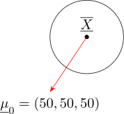
So \(\underline {\mu }_0=\begin {pmatrix} 50, & 50, & 50\\ \end {pmatrix}'\) is not within the confidence \((95\%)\) region.

6.

Find the \(90\%\) confidence interval for \(\mu _2-\mu _3\).

Show solution

Solution. \[F_{3,33}(0.90)=\frac {1}{2}(2.28+2.23)=2.255\]

\[\mu _2 - \mu _3 = L'\underline {\mu } = \begin {pmatrix} 0, & 1, & -1\\ \end {pmatrix} \begin {pmatrix} \mu _1\\ \mu _2\\ \mu _3\\ \end {pmatrix} \]

\begin {align*} \overline {X}_2-\overline {X}_3 & \pm \sqrt {\frac {p(n-1)}{n-p}F_{p,n-p,1-\alpha }\times \frac {S_{22}-2S_{23}+S_{33}}{36}}\\\\ 69.75 - 68.05 & \pm \sqrt {\frac {3\times 35}{33}\times 2.255\times \frac {422.879-2(29.929)+147.897}{36}}\\ \implies \quad 1.69 & \pm \sqrt {7.175 \times 14.192167}\\ \implies \quad 1.69 & \pm 10.0910\\ & \equiv (-8.401,11.781)\\ \end {align*}

Question: What implications does this interval have on \(H_0:\mu _2=\mu _3\) vs \(H_a:\mu _2\neq \mu _3\).

Show solution

Solution. Take \(\underline {a}=(1,1,0)'\). Then \(\underline {a}'\underline {\mu }=3\) and \(\underline {a}'\Sigma \underline {a} = 4+3+2(1) = 9\), so \(X_1+X_2\sim N(3,9)\).

\(X_3\) is independent of \((X_1,X_2)\) because the corresponding off-diagonal block of \(\Sigma \) is zero and the vector is jointly normal. Without joint normality the zero covariances would not be enough.

Show solution

Solution. Considering each variable separately ignores the correlations. If the variables are strongly positively correlated, the joint distribution concentrates near a line, and a point that is moderately high on some variables and moderately low on others lies far off that line while remaining unremarkable in every margin. The Mahalanobis distance measures departure in the metric of \(\Sigma ^{-1}\) and therefore sees it.

This is the multivariate outlier that univariate screening cannot find, and it is the practical argument for the ellipsoidal regions of this section over a box of individual intervals.

Questions on this section

Stuck on something here? Ask below and it stays attached to this topic.