7.1 Fisher’s Discriminant Function
Fishers approach does not assure a particular distribution but rather assures equal covarince
matrix.
It transforms multivariate observations \(X\) to univariate observations \(Y\) such that \(Y's\) derivated
from one population as separated as much as possible from one another population \(\pi _1\) and
\(\pi _2\).
Let \(\underline {Y}= L'\underline {X}\) be a linear combination of \(X's\). The linear combinations transforms from the first population into the
univariate data set
\[Y_{11}, Y_{12}, \ldots , Y_{1n}\]
and transform \(x's\) in the second population into \(y_{21}, y_{22},\ldots , y_{2m}\).
The ideal is to look for \(L\) which will separate \(\overline {Y}_1\) and \(\overline {Y}_2\), an illustration is given below.
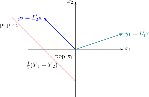
In the diagram \(Y_1 = L'_1\underline {X}\) leads to a population discrimination rule because it is difficult to tell the two
population apart. \(Y_2 = \underline {L}'_2\underline {X}\), reasonable separates the two populations.
The separation of the two sets univariate \(Y_i'\)s is assessed in terms of \(\overline {Y}_1 - \overline {Y}_2\) expressed is \(S.D\) units (standard
deviation).
i.e Separation \(\displaystyle {\frac {|\overline {Y}_1-\overline {Y}_2|}{S_Y}}\) , where \(S_Y\) is such that \begin {align*} S^2_y & = S^2\\ & = \frac {\sum \limits ^{n_1}_{j=1}(Y_{1j}-\overline {Y}_1 )^2 + \sum \limits ^{n_2}_{j=1}(Y_{2j}-\overline {Y}_2)^2}{n_1+n_2-2}\\\\ & = \frac {(n_1-1)S^2_1 + (n_2-1)S^2_1}{n_1+n_2-2}\tag {2} \end {align*}
The task is to select \(L\) which achieves maximum separation with sample means \(\overline {Y}_1\) and \(\overline {Y}_2\).
Result 7.1. The vector \(\displaystyle {L' = \big (\overline {\underline {X}_1}-\overline {\underline {X}_2}\big )'S^{-1}_p}\) can be shown to be the desired choice which achieves maximum
separation between \(\overline {Y}_1\) and \(\overline {Y}_2\).
Result 7.2. Given \(\displaystyle {L' = \big (\overline {\underline {X}_1}-\overline {\underline {X}_2}\big )'S^{-1} = d'S^{-1}}\) choice of \(L\) for the maximum of the separation \(\displaystyle {\frac {|\overline {Y}_1-\overline {Y}_2|}{S_y}}\) is also the maximum of \(D^2\) (distance)
\begin {align*} D^2 & = \max \frac {\big (\overline {Y}_1-\overline {Y}_2\big )^2}{S^2_y}=\max \frac {\big (\widehat {L}'\overline {\underline {X}_1}-\widehat {L}'\overline {\underline {X}_2}\big )^2}{\widehat {L}'S_p\widehat {L}}\\\\ & = \frac {\big (\widehat {L}'\big (\overline {\underline {X}_1}-\overline {\underline {X}_2}\big )^2}{\widehat {L}'S_p\widehat {L}} = \frac {\big (\widehat {L}'d\big )^2}{\widehat {L}'S_p\widehat {L}}\\\\ & = \frac {\big (\widehat {L}'d\big )\big (\widehat {L}'d\big )}{\widehat {L}'S_p\widehat {L}}=\frac {\big (d'S_p^{-1}d\big )\big (d'S_p^{-1}d\big )}{d'S^{-1}_pS_pS^{-1}_pd}\\\\ & = \frac {\big (d'S^{-1}_pd\big )\big (d'S_p^{-1}d\big )}{d'S^{-1}_pd}\\\\ & = \big (d'S^{-1}_pd\big )\tag {3} \end {align*}
\(D^2\) is often used for discrimination \(y_{1j}=\widehat {L}\underline {X}_{1j}\) \(, y_{2j}=\widehat {L}'\underline {X}_{2j}\)
\begin {align*} \text {Pooled}\rightarrow S^2_y & = \frac {\sum \limits ^{n_1}_{j=1}\big (Y_{1j}-\overline {Y}_1\big )^2 + \sum \limits ^{n_2}_{j=1}\big (Y_{2j}-\overline {Y}_2\big )^2}{n_1+n_2-2}\\\\ & = \frac {\sum \limits ^{n_1}_{j=1}\Big (\widehat {L}'\underline {X}_{1j}-\widehat {L}'\overline {\underline {X}_1}\Big )^2 + \sum \limits ^{n_2}_{j=1}\Big (\widehat {L}'\underline {X}_{2j}-\widehat {L}'\overline {\underline {X}_2}\Big )^2}{n_1+n_2-2}\\\\ & = \frac {\sum \limits ^{n_1}_{j=1}\big (\widehat {L}'\underline {X}_{1j}-\widehat {L}'\overline {\underline {X}_1}\big )\big (\widehat {L}'\underline {X}_{1j}-\widehat {L}'\overline {\underline {X}_2}\big )' + \sum \limits ^{n_2}_{j=1}\big (\widehat {L}'\underline {X}_{2j}-\widehat {L}'\overline {\underline {X}_2}\big )\big (\widehat {L}'\underline {X}_{2j}-\widehat {L}'\overline {\underline {X}_2}\big )'}{n_1 + n_2 -2}\\\\ & = \frac {\sum \limits ^{n_1}_{j=1}\widehat {L}'\big (\underline {X}_{1j}-\overline {\underline {X}_1}\big )\big (\underline {X}_{1j}-\overline {\underline {X}_1}\big )'\widehat {L}+ \sum \limits ^{n_2}_{j=1}\widehat {L}'\big (\underline {X}_{2j}-\overline {\underline {X}_2}\big )\big (\underline {X}_{2j}-\overline {\underline {X}_2}\big )'\widehat {L}}{n_1 + n_2 - 2}\\\\ & = \frac {\widehat {L}'\Big [\sum \limits ^{n_1}\big (\underline {X}_{1j}-\overline {\underline {X}_1}\big )\big (\underline {X}_{1j}-\overline {\underline {X}_1}\big )' + \sum \limits ^{n_2}\big (\underline {X}_{2j}-\overline {\underline {X}_2}\big )\big (\underline {X}_{2j}-\overline {\underline {X}_2}\big )'\Big ]}{n_1 + n_2 -2}\\\\ & = \widehat {L}'\Bigg [\frac {(n_1-1)S_1 + (n_2-1)S_2}{n_1 + n_2 -2}\Bigg ]\widehat {L}\\\\ & = \underbrace {\widehat {L}'}_{d'S^{-1}_p} S_p \underbrace {\widehat {L}}_{S^{-1}_pd}\\\\ \end {align*}
Example 7.3. Budges and a test a system for obtained blood measured. There were interested in whether the system gave results consisting with means hemoglobin (Hb) an packed call value (PCV) for men and women random blood samples from 14 females and 15 males where obtained (Hb) and (PCV) were measured using the new system. Below is partial data set from for males and females.
| Females | Males | ||
| Hb | PCV | Hb | PCV |
| 15.5 | 0.45 | 14.0 | 0.41 |
| 13.6 | 0.42 | 15.3 | 0.45 |
| 13.5 | 0.44 | 13.5 | 0.43 |
| 13.0 | 0.395 | 15.8 | 0.46 |
| 13.3 | 0.395 | 15.0 | 0.43 |
\[\text {Calculate}\quad D^2\]
Data
\[\text {Females}:\quad \overline {\underline {X}_1}= \begin {pmatrix} 13.929\\ &\\ 0.41679\\ \end {pmatrix} , S_1 = S_F= \begin {pmatrix} 2.425275 & 0.040676\\ &\\ 0.040676 & 0.000887\\ \end {pmatrix} \]
\[\text {Males:}\quad \overline {\underline {X}_2}= \begin {pmatrix} 15.553\\ &\\ 0.4467\\ \end {pmatrix} , S_2 = S_M = \begin {pmatrix} 1.298381 & 0.014798\\ &\\ 0.014798 & 0.000320\\ \end {pmatrix} \]
\[S_p = \frac {(n_F-1)S_F + (n_M-1)S_M}{n_F + n_M -2}= \begin {pmatrix} 0.1378870 & 0.0020542\\ &\\ 0.0020542 & 0.000447\\ \end {pmatrix} \]
\[\implies \quad S^{-1}_p= \begin {pmatrix} 23.0 & -1056.5\\ &\\ -1056.5 & 70920.0\\ \end {pmatrix} \]
\begin {align*} \underline {d} & = \overline {X}_F - \overline {X}_M = \begin {pmatrix} 13.929 - 15.553\\ &\\ 0.41679 - 0.4467\\ \end {pmatrix}\\\\ & = \begin {pmatrix} -1.624\\ &\\ -0.0299\\ \end {pmatrix}\\ \end {align*}
\begin {align*} D^2 & = \underline {d}'S^{-1}_p \underline {d}\\\\ & = \begin {pmatrix} -1.624\\\ &\\ -0.0299\\ \end {pmatrix}' \begin {pmatrix} 23.0 & -1056.5\\ &\\ -1056.5 & 70920.3\\ \end {pmatrix} \begin {pmatrix} -1.624\\\ &\\ -0.0299\\ \end {pmatrix}\\\\ & = 21.461\\\\\ \end {align*}
Questions on this section
Stuck on something here? Ask below and it stays attached to this topic.