2.1 Introduction
Let \(X_1, \, \cdots \, , \, X_n\) be a random sample from the model \(\{f_{\theta }(x):\, \theta \in \Omega \}\) then
- 1.
- the likelihood function of \(X_1, \, \cdots \, , \, X_n\) is given by \[L(\theta ) = L(\theta , x) = \prod ^n_{i = 1} f_{\theta }(x_i)\]
- 2.
- the log likelihood function of \(X_1, \, \cdots \, , \, X_n\) is give by \[\mathcal {L}(\theta ) = \mathcal {L}(\theta ,x) = \log L(\theta , x)\]
- 3.
- the score function is given by \[S(\theta ) = S(\theta , x) = \frac {\partial }{\partial \theta }\mathcal {L}(\theta ,x)\]
- 4.
- the function \[I(\theta ) = I(\theta ,x) = \frac {-\partial }{\partial \theta }S(\theta ,x) = \frac {-\partial ^2}{\partial \theta ^2}\mathcal {L}(\theta ,x)\] is called the information function of \(X_1, \, \cdots \, , \, X_n\).
- 5.
- the function \(J(\theta ) = E_{\theta }\left [I(\theta , X)\right ]\) is called the Fisher or expected information function
- 6.
- a value \(\widehat {\theta } = \widehat {\theta }(x)\) which maximizes the likelihood function \(L(\theta )\) is called a maximum likelihood estimate (ML-estimate) for \(\theta \). \(\, \widehat {\theta } = \widehat {\theta }(x)\) is called a maximum likelihood estimator (ML-estimator) for \(\theta \).
Note. In many cases, \(\widehat {\theta }\) is found by solving the score equation \(S(\theta ) = 0\) and checking that \(I(\widehat {\theta }) > 0\).
Example 2.1.1. If \(X_1, \, \cdots \, , \, X_n\) is a random sample from the model \(\{f_{\theta }(x):\, \theta \in \Omega \}\). Show that both the Score function and information function are sums of \(n\) terms of identical form.
Solution. \[L(\theta ) = \prod ^n_{i = 1}f_{\theta }(x_i)\] \[\mathcal {L}(\theta ) = \log \prod ^n_{i = 1} f_{\theta }(x_i) = \sum ^n_{i = 1} \log f_{\theta }(x_i)\] \begin {align*} S(\theta ) & = \frac {\partial }{\partial \theta }\mathcal {L}(\theta ) = \frac {\partial }{\partial \theta }\sum ^n_{i = 1} \log f_{\theta }(x_i) = \sum ^n_{i=1} \frac {\partial }{\partial \theta }\log f_{\theta }(x_i) = \sum ^n_{i = 1} \frac {\frac {\partial }{\partial \theta } \, f_{\theta } (x_i)}{f_{\theta }(x_i)} \end {align*}
a sum of \(n\) terms of identical form. \begin {align*} I(\theta ) & = \frac {-\partial }{\partial \theta }\, S(\theta )\\ & =\frac {-\partial }{\partial \theta }\sum ^n_{i = 1} \frac {\frac {\partial }{\partial \theta } \, f_{\theta }(x_i)}{f_{\theta }(x_i)}\\ & = -\sum ^n_{i = 1} \frac {f_{\theta }(x_i)\, \frac {\partial ^2}{\partial \theta ^2}f_{\theta }(x_i) \, - \, \frac {\partial }{\partial \theta }f_{\theta }(x_i)\, \frac {\partial }{\partial \theta }f_{\theta }(x_i)}{\left (f_{\theta }(x_i)\right )^2}\\ & = \sum ^n_{i = 1}\frac {\left (\frac {\partial }{\partial \theta }f_{\theta }(x_i)\right )^2\, - \, f_{\theta }(x_i)\, \frac {\partial ^2}{\partial \theta ^2}\, f_{\theta }(x_i)}{\left (f_{\theta }(x_i)\right )^2}\\ & = \sum ^n_{i = 1}\left [\left (\frac {\frac {\partial }{\partial \theta }f_{\theta }(x_i)}{f_{\theta }(x_i)}\right )^2 \, - \, \frac {\frac {\partial ^2}{\partial \theta ^2}f_{\theta }(x_i)}{f_{\theta }(x_i)}\right ] \end {align*}
a sum of \(n\) terms of identical form. □
Example 2.1.2. Let \(X_1, \, \cdots \, , \, X_n\) be a random sample from the \(POI(\theta )\) distribution. Find the Fisher information and compare it to the variance of the M.L estimator \(\widehat {\theta }\).
Solution. \begin {align*} f_{\theta }(x) & = \frac {e^{-\theta }\, \theta ^x}{x!} = \prod ^n_{i = 1}\frac {e^{-\theta }\, \theta ^{x_i}}{x_i!} = \frac {e^{-n\theta }\, \theta ^{\sum ^n_{i = 1} x_i}}{\prod ^n_{i = 1} x_i!}. \end {align*}
\[\mathcal {L}(\theta ) = \log L(\theta ) = -n\theta + \sum ^n_{i = 1} x_i - \log \prod ^n_{i = 1} x_i!\] \[S(\theta ) = \frac {\partial \mathcal {L}}{\partial \theta } = -n + \frac {\sum ^n_{i = 1} x_i}{\theta }\] \(S(\theta ) = 0\) \[-n + \frac {\sum ^n_{i = 1} x_i}{\theta } = 0\] \[\implies \hspace {0.5cm} n = \frac {\sum ^n_{i = 1} x_i}{\theta }\hspace {0.5cm}\implies \hspace {0.5cm} \theta = \frac {1}{n} \sum ^n_{i = 1} x_i\] \[\widehat {\theta } = \overline {X}.\]
\[I(\theta ) = -\frac {\partial ^2\mathcal {L}}{\partial \theta ^2} = -\left (\frac {-\sum ^n_{i =1} x_i}{\theta ^2}\right ) = \frac {\sum ^n_{i = 1} x_i}{\theta ^2}.\] \begin {align*} J(\theta ) & = E\left [I(\theta , X)\right ] = E\left [\frac {1}{\theta ^2}\sum ^n_{i = 1} X_i\right ] = \frac {1}{\theta ^2}\, \sum ^n_{i = 1} E(X_i) = \frac {1}{\theta ^2}\, \sum ^n_{i = 1}\theta = \frac {n\theta }{\theta ^2} =\frac {n}{\theta }. \end {align*}
\[\var (\widehat {\theta }) = \var (\overline {X}) = \frac {\theta }{n}.\]
\[\text {i.e}\hspace {0.3cm} \var (\widehat {\theta }) = \frac {1}{J(\theta )} = \left [J(\theta )\right ]^{-1}.\] □
Note. If \(X_1, \, \cdots \, , \, X_n\) is a random sample from \(f_{\theta }(x)\) then
\begin {align*} J(\theta ) & = E\left [-\frac {\partial ^2}{\partial \theta ^2}\, \sum ^n_{i = 1} \log \, f_{\theta }(X_i)\right ] = \sum ^n_{i = 1} E\left [\frac {-\partial ^2}{\partial \theta ^2} \, \log f_{\theta }(X_i)\right ] = n\, E\left [\frac {-\partial ^2}{\partial \theta ^2}\, \log f_{\theta }(X)\right ]. \end {align*}
E.G: In the above example \[L_1(\theta ) = \frac {e^{-\theta }\, \theta ^x}{x!}\]
\[\mathcal {L}_1 (\theta ) = -\theta + x\, \log x - \log x!\]
\[S_1(\theta ) = \frac {\partial \mathcal {L}_1}{\partial \theta } = -1 + \frac {x}{\theta }.\]
\[I_1(\theta ) = \frac {-\partial ^2\mathcal {L}_1}{\partial \theta ^2} = -\left (\frac {-x}{\theta ^2}\right ) = \frac {x}{\theta ^2}.\] \begin {align*} J_1(\theta ) & = E\left [I_1(\theta , X)\right ) = E\left (\frac {X}{\theta ^2}\right ) =\frac {E(X)}{\theta ^2} = \frac {\theta }{\theta ^2} =\frac {1}{\theta }. \end {align*}
\(J_1(\theta ) = 1/\theta \) \[\therefore \hspace {0.5cm} J(\theta ) = n\, J_1(\theta ) = \frac {n}{\theta }\hspace {0.3cm}\text {Ans}.\]
Problem 2.1.1. Suppose that \(X\thicksim BIN(n,\theta )\) and we observe \(X\). Find the M.L estimator of \(\theta \), the score function and the Fisher information.
Show solution
Solution. \[\log L(\theta ) = \log \binom {n}{x} + x\log \theta + (n-x)\log (1-\theta ).\] Differentiating gives the score \[S(\theta ,X) = \frac {X}{\theta } - \frac {n-X}{1-\theta } = \frac {X-n\theta }{\theta (1-\theta )} .\] Setting it to zero gives \(X(1-\theta )=(n-X)\theta \), that is \(X=n\theta \), so \[\widehat {\theta } = \frac {X}{n}.\] For the information, \(\partial ^{2}\log L/\partial \theta ^{2} = -X/\theta ^{2} - (n-X)/(1-\theta )^{2}\), and since \(E(X)=n\theta \), \[I(\theta ) = -E\left [\frac {\partial ^{2}\log L}{\partial \theta ^{2}}\right ] = \frac {n\theta }{\theta ^{2}} + \frac {n(1-\theta )}{(1-\theta )^{2}} = \frac {n}{\theta } + \frac {n}{1-\theta } = \frac {n}{\theta (1-\theta )} .\] Note that \(\var \left (\widehat {\theta }\right )=\theta (1-\theta )/n = 1/I(\theta )\): the estimator attains the information bound exactly, which the form of the score — affine in \(X\) — already predicted.
Problem 2.1.2. Suppose that \(X\thicksim NB(k,\theta )\) and we observe \(X\). Find the M.L estimator of \(\theta \), the Score function and the Fisher information.
Show solution
Solution. With \(P_{\theta }(X=x)=\binom {x+k-1}{x}\theta ^{k}(1-\theta )^{x}\), \[\log L(\theta ) = \text {const} + k\log \theta + X\log (1-\theta ),\] so the score is \[S(\theta ,X) = \frac {k}{\theta } - \frac {X}{1-\theta } .\] Setting it to zero, \(k(1-\theta )=X\theta \), giving \[\widehat {\theta } = \frac {k}{k+X}.\] Since \(\partial ^{2}\log L/\partial \theta ^{2} = -k/\theta ^{2} - X/(1-\theta )^{2}\) and \(E(X)=k(1-\theta )/\theta \), \[I(\theta ) = \frac {k}{\theta ^{2}} + \frac {k(1-\theta )}{\theta (1-\theta )^{2}} = \frac {k}{\theta ^{2}} + \frac {k}{\theta (1-\theta )} = \frac {k}{\theta ^{2}(1-\theta )} .\] Here the score is not affine in \(\widehat {\theta }\), and indeed the maximum likelihood estimator is biased — its expectation exceeds \(\theta \) — so the information bound is not attained at finite \(k\).
Example 2.1.3. Let \(X_1, \, \cdots \, , \, X_n\) be a random sample from the \(UNIF(0,\theta )\) distribution. Find the M.L estimator of \(\theta \).
Solution. \(f_{\theta }(x) = \frac {1}{\theta }\hspace {0.3cm}, \hspace {0.3cm} 0 < x < \theta \) \begin {align*} L(\theta ) & = \frac {1}{\theta ^n}\hspace {0.3cm} , \hspace {0.3cm} 0< x_{(1)}\, , \, \cdots \, ,\, x_{(n)} < \theta \\ & = \frac {1}{\theta ^n}\hspace {0.3cm}, \hspace {0.3cm}0 < x_{(1)} < x_{(n)} < \theta \\ & = \frac {1}{\theta ^n}\, I(X_{(1)}> 0)\, I(X_{(n)} < \theta ) \end {align*}
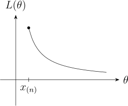
Therefore \(\, \widehat {\theta } = X_{(n)}\). □
Problem 2.1.3. Let \(X_1, \, \cdots \, , \, X_n\) be a random sample from a distribution with pdf \[f_{\theta }(x) = \theta \, x^{\theta - 1}\hspace {0.3cm} , \hspace {0.3cm} 0 < x < 1\hspace {0.2cm}, \hspace {0.3cm} \theta > 0.\] Find the M.L estimator of \(\theta \), the scored function and the Fisher information.
Show solution
Solution. \[\log L(\theta ) = n\log \theta + (\theta -1)\sum _{i=1}^{n}\log X_i ,\] so the score is \[S(\theta ,X) = \frac {n}{\theta } + \sum _{i=1}^{n}\log X_i .\] Setting it to zero and writing \(T=-\sum _{i=1}^{n}\log X_i>0\), \[\widehat {\theta } = \frac {n}{T} = \frac {-n}{\sum _{i=1}^{n}\log X_i}.\] The second derivative is \(-n/\theta ^{2}\), which is already free of the data, so \[I_n(\theta ) = \frac {n}{\theta ^{2}},\] that is \(1/\theta ^{2}\) per observation.
Comparing with the earlier problem on this same density: the UMVUE was \((n-1)/T\) while the maximum likelihood estimator is \(n/T\). The latter is biased upwards by a factor \(n/(n-1)\), and the two agree to first order in \(n\).
Problem 2.1.4. Suppose \(X_1, \, \cdots \, , \, X_n\) is a random sample from the \(UNIF(\theta , \theta + 1)\) distribution. Show that the M.L estimator of \(\theta \) is not unique.
Show solution
Solution. The likelihood is \[L(\theta ) = \prod _{i=1}^{n} I\left (\theta <x_i<\theta +1\right ) = I\left (x_{(n)}-1 < \theta < x_{(1)}\right ),\] which takes only the values \(0\) and \(1\). It equals \(1\) for every \(\theta \) in the interval \(\left (x_{(n)}-1,\ x_{(1)}\right )\) and \(0\) outside it.
Since the likelihood is constant on that interval, every point of it maximises the likelihood equally well. The interval has positive length whenever the sample range is less than one, which happens with probability one, so the maximum likelihood estimator is not unique — there is a continuum of them. Common conventions pick \(x_{(n)}-1\), or \(x_{(1)}\), or the midpoint \(\left (x_{(1)}+x_{(n)}-1\right )/2\), but nothing in the likelihood principle prefers any of them.
Note. This is the standard warning that “the” maximum likelihood estimator is a figure of speech. Uniqueness needs an argument, and here there is none to be had: the data restrict \(\theta \) to an interval and say nothing whatever about where in that interval it lies.
Theorem 2.1.4 (INVARIANCE PROPERTY). If \(\widehat {\theta }\) is the M.L estimator of \(\theta \) and \(\tau (\theta )\) is a function of \(\theta \), then \(\tau (\widehat {\theta })\) is the M.L estimator of \(\tau (\theta )\).
Example 2.1.5. Let \(X_1, \, \cdots \, , \, X_n\) be a random sample from the \(PIO(\theta )\) distribution. Find the M.L estimator of \(\tau (\theta ) = e^{-\theta }\).
Solution. From example 2.1.2, \(\widehat {\theta } = \overline {X}\).
By theorem 2.1.8 \(\widehat {\tau } = e^{-\overline {X}}\, \) is the M.L estimator of \(\tau (\theta ) = e^{-\theta }\). □
Questions on this section
Stuck on something here? Ask below and it stays attached to this topic.