Solution. \[f_{\theta }(x) = \underbrace {C(\theta )\, \exp \left \{\sum ^k_{j = 1} q_j(\theta )\, T_j(x)\right \}}_{g\left (T(X), \theta \right )}\, \underbrace {h(x)}_{h(x)}\] where \(T(X) = (T_1(X), \, \cdots \, , \, T_k(X))\). Therefore by the Factorization Theorem \(T(X)\) is a sufficient statistic. □

Solution. \(X\, \thicksim \, BIN(n,\theta )\) \begin {align*} f_{\theta }(x) & = \binom {n}{x}\, \theta ^x\, (1 - \theta )^{n-x}\hspace {0.3cm} , \hspace {0.6cm} x = 0, \, 1, \, \cdots \, , \, n\\ & = (1 - \theta )^n\, \left (\frac {\theta }{1 - \theta }\right )^x\, \binom {n}{x}\\ & = (1 - \theta )^n\, \exp \left \{\log \left (\frac {\theta }{1 - \theta }\right )^x\right \}\, \binom {n}{x}\\ & = (1 - \theta )^n\, \exp \left \{x\, \log \left (\frac {\theta }{1 - \theta }\right )\right \}\, \binom {n}{x}\\ & = \underbrace {(1 - \theta )^n}_{C(\theta )}\, \exp \Bigg \{\underbrace {\left [\log \left (\frac {\theta }{1 - \theta }\right )\right ]}_{q(\theta }\, \underbrace {x}_{Tx)}\Bigg \} \, \underbrace {\binom {n}{x}}_{h(x)}. \end {align*}

\(\therefore f_{\theta }(x)\) is a member of the exponential family and the natural sufficient statistic is \(T(X) = X\). □

Solution. \(X\, \thicksim \, POI(\theta )\) \begin {align*} f_{\theta }(x) & = \frac {e^{-\theta }\, \theta ^x}{x!}\hspace {0.6cm}, \hspace {0.5cm} x = 0, \, 1, \, \cdots \hspace {0.3cm} \theta > 0 \\ & = e^{-\theta }\, \exp \left (\log \theta ^x\right )\, \frac {1}{x!}\\ & = \underbrace {e^{-\theta }}_{C(\theta )}\, \exp \Bigg \{\underbrace {\left (\log \theta \right )}_{q(\theta )}\, \cdot \, \underbrace {x}_{T(x)}\Bigg \}\, \underbrace {\frac {1}{x!}}_{h(x)} \end {align*}

\(\therefore \, f_{\theta }(x)\) is a member of the exponential family and the natural sufficient statistic is \(T(X) = X\).
\(\therefore \,\) by Theorem 1.6.4 \((X_1, \, \cdots \, , \, X_n)\) has an exponential family (EF) distribution and the natural sufficient statistic is \(T(X) = \sum ^n_{i = 1} X_i\).

OR \begin {align*} f_{\theta }(x_1, \, \cdots \, , \, x_n) & = \prod ^n_{i = 1} \frac {e^{-\theta }\, \theta ^{x_i}}{x_i!} = e^{-n\theta }\, \theta ^{\sum ^n_{i = 1} x_i}\, \prod ^n_{i = 1} \frac {1}{x_i!}\\ & = \underbrace {e^{-n\theta }}_{C(\theta )}\, \exp \Bigg \{\underbrace {\left (\log \theta \right )}_{q(\theta )}\, \underbrace {\sum ^n_{i = 1} x_i}_{T(X)}\Bigg \}\, \underbrace {\prod ^n_{i = 1}\frac {1}{x_i!}}_{h(x)}. \end {align*} □

Solution. From example 1.6.3 \[f_{\theta }(x) = (1 - \theta )^n\, \exp \left \{\left [\log \left (\frac {\theta }{1 - \theta }\right )\right ]\, x\right \}\, \binom {n}{x}.\] Let \(\, \eta = \log \left (\frac {\theta }{1 - \theta }\right ) = q(\theta )\) \begin {align*} 0 &< \theta < 1,\\ 0 & < \frac {\theta }{1 - \theta } < \infty \\ -\infty & < \eta < \infty \end {align*}

We make \(\theta \) the subject \begin {align*} e^{\eta } & = \frac {\theta }{1 - \theta }\\ \theta & = \frac {e^{\eta }}{1 + e^{\eta }}\\ 1 - \theta & = \frac {1}{1 + e^{\eta }} \end {align*}

The natural parameter space is \[\Omega _{\eta } = \left \{\eta :\, -\infty < \eta < \infty \right \}\] Therefore the canonical form is \[f_{\eta }(x) = \left (\frac {1}{1 + e^{\eta }}\right )^n\, \exp \left \{\eta \, x \right \}\, \binom {n}{x}\] no linear constraints on \(T(X) = X\) or \(\eta \) and \(\Omega _{\eta }\) contains a 1-dimensional rectangle.
\(\therefore \, X\, \thicksim \, BIN(n,\theta )\) has a REF distribution. □

Solution. \(X\, \thicksim \, N(\mu , \sigma ^2)\hspace {0.3cm} , \hspace {0.3cm} \theta = (\mu , \sigma ^2)\) \[\Omega = \left \{(\mu , \sigma ^2):\, -\infty < \mu < \infty , \, \, \sigma ^2 > 0\right \}\] \begin {align*} f_{\theta }(x) & = \frac {1}{\sqrt {2\pi \sigma ^2}}\, e^{-\frac {1}{2\sigma ^2}(x - \mu )^2}\\ & = \frac {1}{\sigma ^2}\, e^{-\frac {1}{2\sigma ^2}(x^2 - 2\mu \, x + \mu ^2)}\, \frac {1}{\sqrt {2\pi }}\\ & = \underbrace {\frac {1}{\sigma ^2}}_{C(\theta )}\, e^{-\frac {\mu ^2}{2\sigma ^2}}\, \exp \Bigg \{\underbrace {-\frac {1}{2\sigma ^2}}_{q_1(\theta )}\, \underbrace {x^2}_{T_1(x)}\, + \, \underbrace {\frac {\mu }{\sigma ^2}}_{q_2(\theta }\, \underbrace {x}_{T_2(x)}\Bigg \}\, \underbrace {\frac {1}{\sqrt {2\pi }}}_{h(x)} \end {align*}

\(\therefore \, f_{\theta }(x)\) is a member of the exponential family with natural sufficient statistic
\(\, T(X) = (X, X^2)\).

Let \begin {align*} \eta _1 & = q_1(\theta ) = -\frac {1}{2\sigma ^2}\\\\ \eta _2 & = q_2(\theta ) = \frac {\mu }{\sigma ^2} \end {align*}

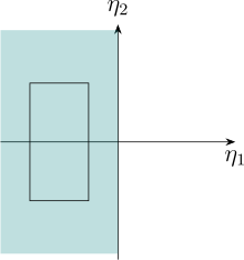
The natural parameter space is \[\Omega _{\eta } = \left \{(\eta _1, \eta _2):\, \eta _1 < 0, \, \, -\infty < \eta _2 < \infty \right \}\]

-

No linear constraints on \(T_j \, '\)s or \(\eta _j\, '\)s.

-

\(\Omega _{\eta }\) contains a 2-dimensional rectangle

\[f_{\eta }(x) = C(\eta )\, \exp \left \{\eta _1\, x^2 + \eta _2\, x\right \}\, \frac {1}{\sqrt {2\pi }}\] Therefore \(X\) has a REF distribution.
\(\therefore \, (X_1, \, \cdots \, , \, X_n)\) has REF distribution with natural sufficient statistics \[T(X) = \left (\sum ^n_{i = 1}X_i \, , \, \sum ^n_{i = 1} X_i^2\right ).\] \(T(X)\) is a completer sufficient statistic (Theorem 1.6.9).
\(\implies \,\left (\overline {X}\, , \, S^2\right )\) is also a complete sufficient statistic since \(E_{\theta }(\overline {X}) = \mu \) and \(E_{\theta }(S^2) = \sigma ^2\). Therefore \(\overline {X}\) is a \(UMVUE\) of \(\mu \) and \(S^2\) is a \(UMVUE\) of \(\sigma ^2\). □

Solution. \(f_{\theta }(x) = \frac {1}{\sqrt {2\pi \theta ^2}}\, e^{-\frac {1}{2\theta ^2}(x - \theta )^2}\) \[\Omega = \left \{\theta :\, \theta \neq 0\right \}\] \begin {align*} f_{\theta }(x) & = \frac {1}{\sqrt {2\pi \, \theta ^2}}e^{-\frac {1}{2\theta ^2}(x - \theta )^2}\\ & = \frac {1}{|\theta |}\, e^{-\frac {1}{2\theta ^2}(x^2 - 2\theta x + \theta ^2)}\, \frac {1}{\sqrt {2\pi }}\\ & = \underbrace {\frac {1}{|\theta |}}_{C(\theta )}\, \exp \Bigg \{\underbrace {-\frac {1}{2\theta ^2}}_{q_1(\theta )}\, \underbrace {x^2}_{T_2(x)}\, + \, \underbrace {\frac {1}{\theta }}_{q_2(x)}\, \underbrace {x}_{T_2(x)}\Bigg \}\, \underbrace {\frac {e^{-\frac {1}{2}}}{\sqrt {2\pi }}}_{h(x)} \end {align*}

\(\therefore \, \, f_{\theta }(x)\) is a member of the REF with natural sufficient statistic \(T(X) = (X, X^2)\).

In Canonical form \begin {align*} \eta _1 & = q_1(\theta ) = -\frac {1}{2\theta ^2}\\ \eta _2 & = q_2(\theta ) = \frac {1}{\theta } \end {align*}

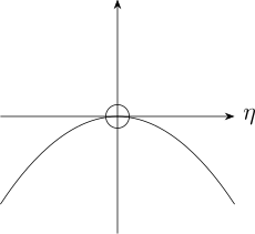
We have that \(\eta _1 = -\frac {1}{2\theta ^2}\) and \(\eta _2 = \frac {1}{\theta }\). \[\implies \hspace {0.5cm} \eta _1 = -\frac {1}{2}\, \eta ^2_2\] \[\Omega _{\eta } = \left \{(\eta _1, \eta _2):\, \eta _1 = -\frac {1}{2}\, \eta ^2_2\, , \, \, \eta _2 \neq 0\right \}.\]

-

Points in \(\Omega _{\eta }\) lie on the curve \(\eta _1 = -\frac {1}{2}\eta ^2_2\).

-

\(\Omega _{\eta }\) doesn’t contain a 2-dimensional rectangle.

\(\therefore \, f_{\theta }(x)\) doesn’t have a REF distribution. □

Solution. \[f_{\theta }(x_1, x_2, x_3) = \frac {n!}{x_1!\, x_2!\, x_3!}\theta _1^{x_1}\, \theta _2^{x_2}\, \theta _3^{x_3}\] \[x_i = 0, \, 1, \, \cdots \] \[x_1 + x_2 + x_3 = n\] \[0 < \theta _i < 1\] \[\theta _1 + \theta _2 + \theta _3 = 1\] \begin {align*} f_{\theta }(x_1, x_2,x_3) & = \exp \left \{\log \left (\theta _1^{x_1}\, \theta _2^{x_2}\, \theta _3^{x_3}\right )\right \}\, \frac {n!}{x_1!\, x_2!\, x_3!}\\ & = \exp \left \{\log \theta _1^{x_1} + \log \theta _2^{x_2} + \log \theta _3^{x_3}\right \}\, \frac {n!}{x_1!\, x_2!\, x_3!}\\ & = \exp \left \{\left (\log \theta _1\right )\, x_1 + \left (\log \theta _2\right )\, x_2 + \left (\log \theta _3\right )\, x_3\right \}\, \frac {n!}{x_1!\, x_2!\, x_3!} \end {align*}

Therefore \(\, f_{\theta }(x_1, x_2, x_3)\) is a member of the EF with natural sufficient statistic
\(T(X) = (X_1, \, X_2, \, X_3) = (T_1, \, T_2, \, T_3).\)
\(T_1 + T_2 + T_3 = n \) - a linear constraint on \(T_j\,'\)s. We therefore rewrite it as \begin {align*} & f_{\theta }(x_1,x_2) = \frac {n!}{x_1!\, x_2!\, (n - x_1 - x_2)!}\, \theta _1^{x_1}\, \theta _2^{x_2}\, (1 - \theta _1 - \theta _2)^{n - x_1 - x_2}\\ & = (1 - \theta _1 - \theta _2)^n\, \exp \left \{\log \left [\left (\frac {\theta _1}{1 - \theta _1 - \theta _2}\right )^{x_1}\, \left (\frac {\theta _2}{1 - \theta _1 -\theta _2}\right )^{x_2}\right ]\right \}\, \frac {n!}{x_1!\, x_2!\, (n - x_1 - x_2)!}\\ & = (1 - \theta _1 -\theta _2)^n\, \exp \left \{x_1\, \log \left (\frac {\theta _1}{1 - \theta _1 - \theta _2}\right ) + x_2\, \log \left (\frac {\theta _2}{1 - \theta _1 - \theta _2}\right )\right \}\, \frac {n!}{x_1!\, x_2!\, (n - x_1 - x_2)!}. \end {align*}

\(\therefore \, f_{\theta }(x_1, x_2)\) is a member of the EF with natural sufficient statistic \(T = (X_1, X_2) = (T_1, T_2)\).
In Canonical form \[\eta _1 = \log \left (\frac {\theta _1}{1 - \theta _1 -\theta _2}\right )\] \[\eta _2 = \log \left (\frac {\theta _2}{1 - \theta _1 - \theta _2}\right )\] \[\Omega _{\eta } = \left \{(\eta _1, \eta _2):\, -\infty < \eta _1 < \infty \, , \, -\infty < \eta _2 < \infty \right \}.\]

-

No linear constraints on \(T_j\,'\)s or \(\eta _j\, '\)s.

-

\(\Omega _{\eta }\) contains a 2-dimensional rectangle.

\[f_{\eta }(x_1, x_2) = \left (\frac {1}{1 + e^{\eta _1} + e^{\eta _2}}\right )^n\, \exp \left \{\eta _1\, x_1 + \eta _2\, x_2\right \}\, h(x)\] is a REF distribution.
Therefore \(T(X) = (X_1, X_2)\) is a complete sufficient statistic. \[E(X_1) = n\theta _1\, , \, E(X_2) = n\theta _2\, ,\, \cov (X_1, X_2) = -n\theta _1\theta _2.\] \[COV(X_1,X_2) = E(X_1X_2) - E(X_1)E(X_2)\] \[-n\theta _1\theta _2 + n\theta _1n\theta _2 - E(X_1X_2)\] \[(n^2 - n)\theta _1\theta _2 = E(X_1X_2)\] \[\frac {E(X_1X_2)}{n(n-1)} = \theta _1 \theta _2\] \[E\left (\frac {X_1X_2}{n(n- 1)}\right ) = \theta _1\theta _2\] \(\therefore \, T(X) = \frac {X_1X_2}{n(n-1)}\, \) is a \(UMVUE\) of \(\tau (\theta ) = \theta _1\theta _2\). □

Solution. \[f_{\theta }(x) = \frac {e^{-\theta }\, \theta ^x}{x!}\,\hspace {0.2cm} , \hspace {0.3cm} x = 0, \, 1,\, 2, \, \cdots \cdots \] Consider \(\, P(X_1 = 0) = e^{-\theta } = \tau (\theta )\).

Let \(\hspace {0.3cm} U = U(X_1) = \begin {cases} 1 & \text {if}\, \, \hspace {0.3cm} X_1 = 0\\ 0 & \text {otherwise}\\ \end {cases} \) \begin {align*} E(U) & = 1\times P(X_1 = 0) + 0\times P(X_1 = 0)\\ & = P(X_1 = 0)\\ & = e^{-\theta }. \end {align*}

\(POI(\theta )\) belongs the the REF distribution. Therefore \(T = \sum ^n_{i = 1} X_i\) is a complete sufficient statistic. \[i.e\hspace {0.5cm} f_{\theta }(x) = e^{-\theta }\, \exp \left \{\left (\log \theta \right )\, x \right \}\, \frac {1}{x!}\] \[\eta = \log \theta \] \[\Omega = \left \{\eta :\, -\infty < \eta < \infty \right \}\]

-

\(\Omega _{\eta }\) contains a 1-dimensional rectangle.

-

No constraints on \(T\) or \(\eta \)

By Lehmaann-Scheff‘es theorem \(E\left [U/T = t\right ]\) is the \(UMVUE\) of \(\tau (\theta )\) \begin {align*} E\left [U/T = t\right ] & = 1\times P(X_1 = 0/T = t) = \frac {P\left (X_1 = 0\,, \, \sum ^n_{i = 1} X_i = t\right )}{P(T = t)}\\ & = \frac {P\left (X_1 = 0\, , \, \sum ^n_{i = 1} X_i = t - 0\right )}{e^{-n\theta }(n\theta )^t/t!}\\ & = \frac {P(X_1 = 0)\, P\left (\sum ^n_{i = 1} X_i = t\right )}{e^{-n\theta }(n\theta )^t/t!}\\ & = \frac {e^{-\theta }\, \frac {e^{-(n - 1)\theta }((n-1)\theta )^t}{t!}}{e^{-n\theta }(n\theta )^t/t!}\\ & = \frac {e^{-n\theta }\, (n - 1)^t}{e^{-n\theta }\, n^t} = \left (\frac {n - 1}{n}\right )^t\, , \hspace {0.3cm} t = 0, \, 1, \, 2, \, \cdots \end {align*}

\(\therefore \, h(T) = \left (1 - \dfrac {1}{n}\right )^T\,\) is the \(UMVUE\) of \(\tau (\theta ) = e^{-\theta }\). □

Solution. \(\tau (\theta ) = \Phi (C - \theta ) = P(X\leq C)\)

Let \(\hspace {0.3cm} U(X_1) = \begin {cases} 1 & \text {if}\hspace {0.2cm} X\leq C\\ 0 & \text {otherwise} \end {cases}\) \[E(U) = P(X\leq C)\] \(N(\theta ,1)\,\) is a REF distribution. Therefore \(T = \sum ^n_{i = 1} X_i \,\) is a complete sufficient statistic.
By Lehmann-Scheffe‘s Theorem \(E(U \mid T = t)\) is the \(UMVUE\) of \(\tau (\theta )\). \[f(x/T= t) = \frac {f(x , t)}{f_T(t)} = \frac {f(x, t-x)}{f_T(t)} = \frac {f(x)\, f(t -x)}{f_T(t)}.\] \[T = \sum ^n_{i = 1} X_i\, \thicksim \, N(n\theta , n)\] \[T - X = \sum ^{n - 1}_{i = 1} X_i \, \thicksim \, N\left ((n - 1)\theta , n - 1\right )\] \begin {align*} & f(X/T = t) = \frac {\frac {1}{\sqrt {2\pi }}\exp \left \{\frac {-1}{2}(x - \theta )^2\right \}\, \cdot \, \frac {1}{\sqrt {2\pi (n - 1)}}\exp \left \{\frac {-1}{2(n-1)}(t - x) - (n - 1)\theta )^2\right \}}{\frac {1}{\sqrt {2\pi n}}\exp \left \{\frac {-1}{2n}(t - n\theta )^2\right \}}\\ & = \frac {\sqrt {n}}{\sqrt {2\pi (n - 1)}}\exp \left \{\frac {-1}{2}\left ((x - \theta )^2 + \frac {1}{n - 1}(t - x - (n - 1)\theta )^2 - \frac {1}{n}(t - n\theta )^2\right )\right \}\\ & = \frac {\sqrt {n}}{\sqrt {2\pi (n - 1)}}\, \exp \left \{\frac {-1}{2}\left ((x - \theta )^2 + \frac {(t - n\theta )^2}{n - 1} - \frac {2(t - \theta n)(x - \theta )}{n - 1} + \frac {(x - \theta )^2}{n - 1} - \frac {(t - n\theta )^2}{n}\right )\right \}\\ & = \frac {\sqrt {n}}{\sqrt {2\pi (n - 1)}}\, \exp \left \{\frac {-n}{2(n - 1)}\left (x^2 - \frac {2tx}{n} + \frac {t^2}{n^2}\right )\right \}\\ & = \frac {\sqrt {n}}{\sqrt {2\pi (n - 1)}}\, \exp \left \{\frac {-n}{2(n-1)}\left (x - \frac {t}{n}\right )^2\right \}\\ & = \frac {1}{\sqrt {2\pi \left (\frac {n - 1}{n}\right )}}\,\exp \left \{\frac {-1}{2\left (\frac {n - 1}{n}\right )}\left (x - \frac {t}{n}\right )^2\right \} \end {align*}

\[X/ T = t\, \thicksim \, N\left (\frac {t}{n}\, , \, \frac {n - 1}{n}\right )\] \begin {align*} E\left (U \mid T = t\right ) & = E\left [I(X\leq C)/ T = t\right ]\\ & = P\left (X \leq C / T = t\right )\\ & = P\left (\frac {X - t/n}{\sqrt {\frac {n - 1}{n}}} \, \leq \, \frac {C - t/n}{\sqrt {\frac {n - 1}{n}}}\right )\\ & = P\left (Z \, \leq \frac {C - t/n}{\sqrt {\frac {n - 1}{n}}}\right )\\ & = \Phi \left (\frac {C - t/n}{\sqrt {\frac {n - 1}{n}}}\right ) \end {align*}

\(\therefore \,\, \Phi \left (\frac {C - t/n}{\sqrt {\frac {n - 1}{n}}}\right )\) is the \(UMVUE\) of \(\tau (\theta ) = P(X\leq C)\). □