Proof. Fix \(\varepsilon >0\) small enough that \([\theta _0-\varepsilon ,\theta _0+\varepsilon ]\subset \Omega \), and write \[\ell _n(\theta ) = \frac {1}{n}\sum _{i=1}^{n}\log f_{\theta }(X_i).\] For each fixed \(\theta \) the summands are independent and identically distributed, so by the weak law of large numbers \[\ell _n(\theta ) - \ell _n(\theta _0) \underset {P}{\longrightarrow } E_{\theta _0}\left [\log \frac {f_{\theta }(X)}{f_{\theta _0}(X)}\right ] = -K(\theta _0,\theta ),\] where \(K(\theta _0,\theta )\) is the Kullback–Leibler divergence. By Jensen’s inequality applied to the strictly concave logarithm, \[E_{\theta _0}\left [\log \frac {f_{\theta }(X)}{f_{\theta _0}(X)}\right ] \;\leq \; \log E_{\theta _0}\left [\frac {f_{\theta }(X)}{f_{\theta _0}(X)}\right ] = \log \int f_{\theta }(x)\,dx = 0,\] with equality only when \(f_{\theta } = f_{\theta _0}\) almost everywhere. Since the model is identifiable, \(K(\theta _0,\theta ) > 0\) for every \(\theta \neq \theta _0\).

Apply this at the two endpoints \(\theta _0 \pm \varepsilon \). With probability tending to one, \[\ell _n(\theta _0) > \ell _n(\theta _0-\varepsilon ) \qquad \text {and}\qquad \ell _n(\theta _0) > \ell _n(\theta _0+\varepsilon ),\] so \(\ell _n\) attains a local maximum at some interior point \(\widehat {\theta _n}\in (\theta _0-\varepsilon ,\theta _0+\varepsilon )\). At an interior maximum of a differentiable function the derivative vanishes, so \(\widehat {\theta _n}\) solves the likelihood equation \(\sum _{i=1}^{n}S_1(\theta ,X_i)=0\). As \(\varepsilon >0\) was arbitrary, \[P\left (\left |\widehat {\theta _n}-\theta _0\right |<\varepsilon \right )\longrightarrow 1 \qquad \text {for every } \varepsilon >0,\] which is exactly \(\widehat {\theta _n}\underset {P}{\longrightarrow }\theta _0\). □

Solution.

(a)

\(f_{\theta }(x) = \theta \, x^{\theta - 1}\) \[L(\theta ) = \prod ^n_{i= 1} \theta \, x_i^{\theta - 1} = \theta ^n\, \left (\prod ^n_{i = 1} x_i\right )^{\theta - 1}.\]

\[\mathcal {L}(\theta ) = n\, \log \theta + (\theta - 1)\, \log \prod ^n_{i = 1} x_i.\]

\[S(\theta ) = \frac {n}{\theta } + \log \prod ^n_{i = 1} x_i.\] \(S(\theta ) = 0\) \[\frac {n}{\theta } + \sum ^n_{i = 1} \log x_i = 0\]

\[\widehat {\theta _n} = \frac {n}{-\sum ^n_{i = 1} \log x_i}\] \(\widehat {\theta } = \frac {n}{T}\) where \(T = -\sum ^n_{i = 1} \log X_i\) is the \(ML\) estimator of \(\theta \).

(b)

\(I(\theta ) = -\left (-\dfrac {n}{\theta ^2}\right ) = \dfrac {n}{\theta ^2}\) \[J(\theta ) = E\left [I(\theta ,X)\right ] = \dfrac {n}{\theta ^2}.\]

\[\sqrt {J\left (\widehat {\theta _n}\right )}\, \left (\widehat {\theta _n} - \theta \right ) \, \underset {D}{\longrightarrow }\, Z\thicksim N(0,1)\]

\[\frac {\widehat {\theta _n} - \theta }{\dfrac {1}{\sqrt {J\left (\widehat {\theta _n}\right )}}}\, \underset {D}{\longrightarrow }\, Z \thicksim N(0,1).\]

An approximate 95\(\%\) C.I for \(\theta \) is given by \[\widehat {\theta _n} \pm 1.96\, \frac {1}{\sqrt {J(\widehat {\theta _n})}}\] \[\frac {n}{T} \pm 1.96\, \sqrt {\frac {1}{\dfrac {n}{\widehat {\theta _n}^2}}}\] \[\frac {n}{T}\pm 1.96 \frac {\widehat {\theta _n}}{\sqrt {n}}\] \[\frac {n}{T} \pm 1.96 \, \frac {\left (\frac {n}{T}\right )}{\sqrt {n}}\] \[\frac {n}{T} \pm 1.96\, \frac {\sqrt {n}}{T}\]

(c)

\(-\log X_i \thicksim ExP\left (\frac {1}{\theta }\right )\) \[T = - \sum ^n_{i = 1} \log X_i \thicksim GAM \left (n, \frac {1}{\theta }\right )\] then \(Y = 2\theta T\thicksim \chi ^2_{2n}\).
Now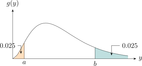

Thus an exact \(95\%\) equal tailed C.I is given as follows: \[P(a < Y < b) = 0.95\] \[P\left (a < 2\theta T < b\right ) = 0.95\] \[P\left (\frac {1}{2T} < \theta < \frac {b}{2T}\right ) = 0.95\] Therefore \(\left [\frac {a}{2T}\, , \, \frac {b}{2T}\right ]\) is an exact \(95\%\) C.I for \(\theta \) where \[a = \chi ^2_{0.025,2n}\] \[b = \chi ^2_{0.975, 2n}\] i.e \[P\left (\chi ^2_{2n} \leq a\right ) = 0.025\] \[P\left (\chi ^2_{2n} \leq b \right ) = 0.975.\]

Solution. From example 2.1.2 \[\widehat {\theta }_n = \overline {X}_n\] \[J(\theta ) = \frac {n}{\theta }\] an approximate \(95\%\) C.I for \(\theta \) is given by \[\widehat {\theta }_n \, \pm \, 1.96\, \sqrt {\dfrac {1}{J(\widehat {\theta }_n)}}\] \[\overline {X}_n \, \pm \, 1.96\, \sqrt {\dfrac {\widehat {\theta }_n}{n}}\] \[\overline {X}_n \, \pm \, 1.96\, \sqrt {\dfrac {\overline {x}_n}{n}}\] By Theorem 2.5.3 \[\sqrt {n}\, \left (\tau (\widehat {\theta }_n) - \tau (\theta )\right ) \, \underset {D}{\longrightarrow }\, N\left (0, \frac {\left (\tau '(\theta )\right )^2}{J_1(\theta )}\right )\] i.e \[T\left (\widehat {\theta }_n\right ) - \tau (\theta ) \, \underset {D}{\longrightarrow }\, N\left (0\, , \, \frac {\left (\tau '(\theta )\right )^2}{J(\theta )}\right )\]

\[\tau (\theta ) = e^{-\theta }\, \implies \, \tau '(\theta ) = - e^{-\theta }\] an approximate \(95\%\) C.I for \(\tau (\theta ) = e^{-\theta }\) is given by \[\tau \left (\widehat {\theta }_n\right )\pm 1.96\, \sqrt {\dfrac {\left (\tau '(\widehat {\theta }_n)\right )^2}{J(\widehat {\theta }_n)}}\]

\[e^{-\overline {x}_n} \, \pm 1.96\, \sqrt {\dfrac {\left (e^{-\widehat {\theta }_n}\right )^2}{n/\widehat {\theta }_n}}\]

\[e^{-\overline {x}} \, \pm \, 1.96\, e^{-\overline {x}}\, \sqrt {\dfrac {\overline {x}_n}{n}}.\] □

Solution. \begin {align*} L(\theta ) & = \prod ^n_{i = 1} e^{-(x_i - \theta )}\hspace {0.3cm} , \hspace {0.6cm} x_1, \, \cdots \, , \, x_n > \theta \\ & = e^{-\sum ^n_{i = 1}(x_i - \theta )}\hspace {0.3cm} , \hspace {0.6cm} x_{(1)} > \theta \\ & = e^{n\theta - \sum ^n_{i = 1} x_i}\hspace {0.3cm} , \hspace {0.6cm} x_{(1)} > \theta \end {align*}

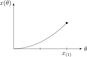
Therefore \(\, \widehat {\theta }_n = X_{(1)}\). \[\widehat {\theta }_n \underset {P}{\longrightarrow } \theta \hspace {0.6cm} \text {if}\hspace {0.6cm} \lim _{n \rightarrow \infty } P\left (\left |\widehat {\theta }_n - \theta \right | > \varepsilon \right ) = 0.\] \begin {align*} P\left (\left |\widehat {\theta }_n - \theta \right | > \varepsilon \right ) & = P\left (\widehat {\theta }_n -\theta > \varepsilon \right ) + P\left (\widehat {\theta }_n - \theta < -\varepsilon \right )\\ & = P(X_{(1)} - \theta > \varepsilon ) + P(X_{(1)} - < -\varepsilon )\\ & = P(X_{(1)} > \varepsilon + \theta ) + P(X_{(1)} < -\varepsilon + \theta ). \end {align*}

Now, let \(Y = X_{(1)}\) \[f_{X_{(1)}}(y) = n\left [1 - F_X(y)\right ]^{n - 1}\, f_X(y)\]

\[F(y) = \int ^y_{\theta } e^{-(x - \theta )}\, dx = -e^{-(x - \theta )}\Big |_{\theta }^y = 1 + e^{-(y - \theta )}.\]

\[f(y) = n \left (e^{-(y - \theta )}\right )^{n - 1}\, e^{-(y - \theta )} = n\, e^{-n(y - \theta )}\hspace {0.3cm} , \hspace {0.5cm} y > \theta .\]

\begin {align*} P\left (\left |X_{(1)} - \theta \right | > \varepsilon \right ) & = \int ^{\infty }_{\theta + \varepsilon } n\, e^{-n(y -\theta )}\, dy \, +\, \underbrace {\int _{-\infty }^{\theta - \varepsilon } n\, e^{-n(y - \theta )}\, dy}_0\\ & =\frac {n\, e^{-n(y - \theta )}}{-n}\Big |_{\theta + \varepsilon }^{\infty }\\ & = - \left (0 - e^{-n(\theta + \varepsilon - \theta )}\right )\\ & = e^{-n\varepsilon }\, \longrightarrow \, 0. \end {align*}

i.e \(\lim _{n\rightarrow \infty } P\left (\left |X_{(1)} - \theta \right | > \varepsilon \right ) = 0\). Therefore \(\, X_{(1)} \underset {P}{\longrightarrow } \theta \) (it is consistent).

Let \(\, T = n\left (\widehat {\theta }_n - \theta \right )\) \begin {align*} F(t) & = P\left (T\leq t\right ) = P\left (n\left (\widehat {\theta }_n - \theta \right ) \leq t\right )\\ & = P\left (X_{(1)} - \theta \leq \frac {t}{n}\right )\\ & = P\left (X_{(1)} \leq \theta + \frac {t}{n}\right )\\ & = \int ^{\theta + \frac {t}{n}}_{\theta } n\, e^{-n(y - \theta )}\, dy\\ & = -e^{-n(y - \theta )}\Big |^{\theta + \frac {t}{n}}_{\theta }\\ & = 1 - e^{-t}. \end {align*}

We find the pdf by differentiating \[f(t) = e^{-t}\hspace {0.5cm} , \hspace {0.4cm} t> 0.\,\,\,\, \text {Therefore}\hspace {0.5cm} T\thicksim EXP(1).\]

A \(95\%\) C.I for \(\theta \) is calculated as follows: \[P(a < n(X_{(1)} - \theta ) < b) = 0.95\] \[P\left (\frac {a}{n} < X_{(1)} - \theta < \frac {b}{n}\right ) = 0.95\] \[P\left (-\frac {a}{n} > \theta - X_{(1)} > -\frac {b}{n}\right ) = 0.95\] \[P\left (-\frac {b}{n} < \theta - X_{(1)} < - \frac {a}{n}\right ) = 0.95\] \[P\left (X_{(1)} - \frac {b}{n} < \theta < X_{(1)} - \frac {a}{n}\right ) = 0.95\] \[\left [X_{(1)} - \frac {b}{n}\, , \, X_{(1)} - \frac {a}{n}\right ].\] where

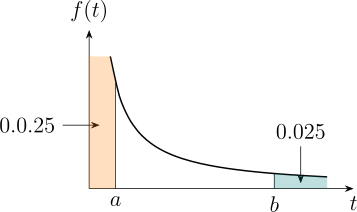
\[F(a) = 1 - e^{-a} = 0.025 \, \implies e^{-a} = 0.975\] \[a = -\log 0.975\]

\[F(b) = 1 - e^{-b} = 0.975 \, \implies e^{-b} = 0.025\] \[b = -\log 0.025.\]

\[\left [X_{(1)} + \frac {\log 0.025}{n} \, , \, X_{(1)} + \frac {\log 0.975}{n}\right ].\] □

Solution. From example 2.2.8 \[J(\theta ) = \begin {pmatrix} n\, \Psi '(\alpha ) & \dfrac {n}{\beta }\\\\ \dfrac {n}{\beta } & \dfrac {n\alpha }{\beta ^2}\\ \end {pmatrix}\]

\[\left |J(\theta )\right | = \frac {n^2\, \alpha \, \Psi '(\alpha }{\beta ^2} - \frac {n^2}{\beta ^2} = \frac {n^2\, \left (\alpha \, \Psi '(\alpha ) - 1\right )}{\beta ^2}.\]

\[\left [J(\theta )\right ]^{-1} = \frac {\beta ^2}{n^2\, \left (\alpha \, \Psi '(\alpha ) - 1\right )}\begin {pmatrix} \dfrac {n\alpha }{\beta ^2} & -\dfrac {n}{\beta }\\\\ -\dfrac {n}{\beta } & n\, \Psi '(\alpha )\\ \end {pmatrix} = \frac {\beta ^2}{n\, \left (\alpha \, \Psi '(\alpha ) - 1\right )}\begin {pmatrix} \dfrac {\alpha }{\beta ^2} & -\dfrac {1}{\beta }\\\\ -\dfrac {1}{\beta } & \Psi '(\alpha )\\ \end {pmatrix}.\]

a \(95\%\) C.I for \(\beta \) is given by \[\widehat {\beta }_n \, \pm \, 1.96\, \sqrt {\var \left (\widehat {\beta }_n\right )}\]

\[\widehat {\beta }_n \, \pm \, 1.96\, \sqrt {\left [J\left (\widehat {\theta }_n\right )\right ]_{22}}\]

\[\widehat {\beta }_n\, \pm \, 1.96\, \sqrt {\dfrac {\widehat {\beta }_n^2\, \Psi '\left (\widehat {\alpha }_n\right )}{n\,\left (\widehat {\alpha }_n\, \Psi \left (\widehat {\alpha }_n\right )\right )^{-1}}}.\]

\[\tau \left (\widehat {\theta }_n\right ) - \tau (\theta ) \, \underset {D}{\longrightarrow }\, W\thicksim MVN\left (0\, , \, D(\theta )^t\, \left [J(\theta )\right ]^{-1}\, D(\theta )\right )\]

\[\tau (\theta ) = \alpha \beta \]

\[D(\theta ) = \begin {pmatrix} \dfrac {\partial \tau }{\partial \alpha }\\\\ \dfrac {\partial \tau }{\partial \beta }\\ \end {pmatrix} = \begin {pmatrix} \beta \\ \alpha \\ \end {pmatrix}.\] \begin {align*} D(\theta )^t\, \left [J(\theta )\right ]^{-1}\, D(\theta ) & = \begin {pmatrix} \beta & \alpha \\ \end {pmatrix} \frac {\beta ^2}{n\, \left (\alpha \, \Psi '(\alpha ) - 1\right )}\begin {pmatrix} \dfrac {\alpha }{\beta ^2} & -\dfrac {1}{\beta }\\\\ -\dfrac {1}{\beta } & \Psi '(\alpha )\\ \end {pmatrix}\, \begin {pmatrix} \beta \\ \alpha \\ \end {pmatrix}\\\\ & = \frac {\beta ^2}{n\, \left (\alpha \, \Psi '(\alpha ) - 1\right )} \begin {pmatrix} \dfrac {\alpha }{\beta } - \dfrac {\alpha }{\beta } && -1 + \alpha \, \Psi '(\alpha )\\ \end {pmatrix}\, \begin {pmatrix} \beta \\ \alpha \\ \end {pmatrix}.\\\\ & = \frac {\beta ^2}{n\, \left (\alpha \, \Psi '(\alpha ) - 1\right )}\, \begin {pmatrix} 0 + \alpha \left (\alpha \, \Psi '(\alpha ) - 1\right )\\ \end {pmatrix}\\\\ & = \frac {\alpha \, \beta ^2}{n} \end {align*}

a \(95\%\) C.I for \(\tau (\theta ) = \alpha \beta \) is given by \[\widehat {\alpha }_n\widehat {\beta }_n\, \pm \, 1.96\, \sqrt {\dfrac {\widehat {\alpha }_n\, \widehat {\beta }_n^2}{n}}.\] □