1.2 Unbiasedness and Mean Square Error
What desirable properties should our estimator have?
- 1.
- Is it estimating the correct parameter?
- 2.
- Is it not consistently too large or too small?
One way of addressing (1) is to study unbiasedness.
Note. We will denote an expected value under the assumed parameter value \(\theta \) by \(E_{\theta }(\cdot )\). Thus \[E_{\theta }\left [h(x)\right ] = \begin {cases} \displaystyle {\int _{\text {all} \, x} h(x)\, f_{\theta }(x)\, dx} & \text {if}\hspace {0.2cm} X\hspace {0.2cm}\text {is continuous}\\\\ \displaystyle {\sum _{\text {all}\, x} h(x)\, f_{\theta }(x)} & \text {if}\hspace {0.2cm} X\hspace {0.2cm} \text {is discrete}\\ \end {cases} \]
Example 1.2.1. Suppose that \(X\) has Cauchy CAU(1,0) distribution show that \(E_{\theta }(X)\) does not exists.
Solution. \(\displaystyle {f_{\theta }(x) = \dfrac {1}{\pi \left (1 + x^2\right )}}\hspace {0.2cm},\hspace {0.5cm} -\infty < x < \infty \) \begin {align*} E_{\theta }\,|x| & = \int ^{\infty }_{-\infty }\frac {\mid x\mid }{\pi \left (1 + x^2\right )}\, dx \\\\ & = \dfrac {2}{\pi }\int ^{\infty }_{0} \frac {x}{1 + x^2}\, dx\\\\ & = \lim _{m \rightarrow \infty } \, \frac {2}{\pi }\int ^{\infty }_0\frac {x}{1 + x^2}\, dx\\\\ & = \lim _{m\rightarrow \infty } \frac {1}{\pi }\, \log \left (1 + x^2\right )\Bigg |^m_0\\\\ & = \infty \end {align*} □
Example 1.2.2. Suppose that \(X\) is a random variable with p.d.f \[f_{\theta }(x) = \dfrac {\theta }{x^{\theta + 1}}\hspace {0.3cm}, \hspace {0.5cm} x\geq 1\] For what values of \(\theta \) do \(E_{\theta }(X)\) and \(\var _{\theta }(X)\) exists?
Solution. \begin {align*} E_{\theta }(X) & = \int _{\text {all}\, x} x\, f_{\theta }(x)\, dx = \int _1^{\infty } x\, \frac {\theta }{x^{\theta + 1}}\, dx = \int _1^{\infty } \theta \, x^{-\theta }\, d\theta \\\\ & = \dfrac {\theta }{1 - \theta } \, x^{1-\theta }\Bigg |^{\infty }_1\hspace {0.3cm}, \hspace {0.5cm} \theta \neq 1\\\\ & = \frac {\theta }{1 - \theta }\, (0 - 1)\hspace {0.3cm}, \hspace {0.5cm} 1 - \theta < 0\\\\ & = \frac {\theta }{1 - \theta }\hspace {0.3cm}, \hspace {0.5cm} \theta > 1 \end {align*}
\[\var _{\theta }(X) = E_{\theta }\left (X^2\right ) - \left [E_{\theta }(X)\right ]^2\]
\begin {align*} E_{\theta }\left (X^2\right ) & = \int _1^{\infty }x^2 \, \frac {\theta }{x^{\theta + 1}}\, dx = \int _1^{\infty } \theta \, x^{1-\theta }\, dx\\\\ & = \dfrac {\theta }{2 - \theta }\, x^{2 - \theta }\Bigg |^{\infty }_{1}\hspace {0.3cm},\hspace {0.5cm} \theta \neq 2\\\\ & = \frac {\theta }{2 - \theta }\, (0 - 1)\hspace {0.3cm}, \hspace {0.5cm} 2-\theta < 0\\\\ & = \frac {\theta }{\theta - 2}\hspace {0.3cm} , \hspace {0.5cm} \theta > 2 \end {align*}
\begin {align*} \var _{\theta }(X) & = E_{\theta }\left (X^2\right ) - \left [E_{\theta }(X)\right ]^2\\\\ & = \dfrac {\theta }{\theta - 2} - \left (\frac {\theta }{\theta - 1}\right )^2 = \frac {\theta }{\theta - 2} - \frac {\theta ^2}{\left (\theta - 1\right )^2}\hspace {0.5cm}\theta \neq 1\, , \, \theta \neq 2\\\\ & = \frac {\theta (\theta - 1)^2 - \theta ^2(\theta - 2)}{(\theta - 1)^2(\theta - 2)}\\\\ & = \frac {\theta \left [\theta ^2 - 2\theta + 1 - \theta ^2 + 2\theta \right ]}{(\theta - 1)^2(\theta - 2)}\\\\ & = \frac {\theta }{(\theta - 1)^2(\theta - 2)}\\\\ \therefore \, \var _{\theta }(X) & = \frac {\theta }{(\theta - 1)^2(\theta - 2)}\hspace {0.3cm}, \hspace {0.5cm} 2<\theta \end {align*} □
Problem 1.2.1. If \(X\thicksim \) GAM\((\alpha \, , \, \beta )\), show that \[E_{\theta }\left (X^p\right ) = \frac {\beta ^p\, \Gamma \left (\alpha + p\right )}{\Gamma (\alpha )}\] For what values of \(p\) does this expectation exist?
Show solution
Solution. The GAM\((\alpha ,\beta )\) density is \[f(x) = \frac {x^{\alpha -1}e^{-x/\beta }}{\beta ^{\alpha }\Gamma (\alpha )},\qquad x>0 .\] Hence \[E\left (X^{p}\right ) = \frac {1}{\beta ^{\alpha }\Gamma (\alpha )}\int _0^{\infty } x^{\alpha +p-1}e^{-x/\beta }\,dx .\] The integral is the normalising constant of a GAM\((\alpha +p,\beta )\) density, so it equals \(\beta ^{\alpha +p}\,\Gamma (\alpha +p)\) whenever \(\alpha +p>0\), and \[E\left (X^{p}\right ) = \frac {\beta ^{\alpha +p}\Gamma (\alpha +p)}{\beta ^{\alpha }\Gamma (\alpha )} = \frac {\beta ^{p}\,\Gamma (\alpha +p)}{\Gamma (\alpha )} .\]
When it exists
The integral converges at the origin only if \(\alpha +p>0\), so the expectation exists precisely for \(p>-\alpha \). Positive moments always exist; negative moments exist only down to \(-\alpha \), which is why \(E(1/X)\) requires \(\alpha >1\) and \(E(1/X^{2})\) requires \(\alpha >2\). Convergence at infinity is never in doubt — the exponential dominates any power.
Problem 1.2.2. Let \(\, m(t) = E\left (e^{tx}\right )\,\) be the moment generating function of a continued random variable \(X\). The function \(m(-t)\) is often called the Laplace Transform of the probability function \(X\). Show that \[E\left (X^{-p}\right ) = \frac {1}{\Gamma (p)}\, \int _0^{\infty }\, m(-t)\, t^{p - 1}\, dt\]
Show solution
Solution. Assume \(X>0\) with probability one and \(p>0\). The key is the integral representation of a negative power: substituting \(u=tx\) in \[\int _0^{\infty } e^{-tx}\,t^{p-1}\,dt = \frac {1}{x^{p}}\int _0^{\infty }e^{-u}u^{p-1}\,du = \frac {\Gamma (p)}{x^{p}}, \qquad x>0 .\] Now start from the right-hand side of the claim and use \(m(-t)=E\left (e^{-tX}\right )\): \[\frac {1}{\Gamma (p)}\int _0^{\infty } m(-t)\,t^{p-1}\,dt = \frac {1}{\Gamma (p)}\int _0^{\infty } E\left (e^{-tX}\right ) t^{p-1}\,dt = \frac {1}{\Gamma (p)}\, E\left [\int _0^{\infty } e^{-tX}t^{p-1}\,dt\right ],\] the exchange of expectation and integral being justified by Tonelli’s theorem, since the integrand is non-negative throughout. By the displayed identity the inner integral is \(\Gamma (p)/X^{p}\), so the whole expression is \[\frac {1}{\Gamma (p)}\,E\left [\frac {\Gamma (p)}{X^{p}}\right ] = E\left (X^{-p}\right ).\]
Note. The result converts a negative moment, which is usually awkward, into an integral of the moment generating function, which is often known in closed form. The requirement \(X>0\) is essential: without it \(X^{-p}\) need not be defined, and \(m(-t)\) need not be finite for all \(t>0\).
1.2.1 Unbiased Estimators
Definition 1.2.3. A statistic \(T(X)\) is an unbiased estimator of \(\theta \) if \(E_{\theta }\left (T(X)\right ) = \theta \,\) for all \(\theta \in \Omega \).
Example 1.2.4. Suppose \(X_i\thicksim \) POI\((i\theta )\, , \hspace {0.3cm} i = 1, \, 2, \, \cdots \, n\,\) independently. Determine whether the estimators \(\, {T_1 = \frac {1}{n} \sum _{i = 1}^{n} \frac {X_i}{i}}\hspace {0.3cm}\) and \(\, {T_2 = \frac {2}{n(n+1)}\sum ^n_{i=1}X_i}\,\) are unbiased estimators of \(\theta \).
Solution. \[ E\left (T_1\right ) \, =\, E\left [\frac {1}{n}\sum _{i = 1}^n\frac {X_i}{i}\right ] = \frac {1}{n}\sum _{i = 1}^n\frac {E\left (X_i\right )}{i}\, = \,\frac {1}{n}\sum ^n_{i = 1}\frac {i\theta }{i}\, =\, \frac {1}{n}\, n\theta \, = \,\theta .\]
\(\therefore \,\, T_1\,\) is an unbiased estimator of \(\theta \).
\begin {align*} E\left (T_2\right ) & = E\left ( \frac {2}{n(n+1)} \, \sum ^n_{i=1} X_i\right ) = \frac {2}{n(n+1)}\sum ^n_{i = 1} E\left (X_i\right )\\ & = \frac {2}{n(n+1)}\sum _{i = 1}^ni\theta \\ & = \frac {2\theta }{n(n+1)}\sum ^n_{i=1}i = \frac {2\theta }{n(n+1)}\cdot \frac {n(n+1)}{2}\\ & = \theta \end {align*}
\(\therefore \,\, T_2\,\) is an unbiased estimator of \(\theta \). □
Note. Unbiased estimator is generally not preserved under transformations. For example, if \(T\) is an unbiased estimator of \(\theta \), then \(T^2\) may be not an unbiased estimator of \(\theta ^2\).
Example 1.2.5. Suppose \(X_1, \, X_2 \cdots \, X_n\) are uncorrelated random variables with \(E(X_i) = \mu \) and \(\var (X_i) = \sigma ^2\, , \hspace {0.3cm} i = 1\, , \, 2\, , \, \cdots \cdots \, , \, n\).
- (i).
- Show that \(\, \displaystyle {T = \frac {1}{n} \sum ^n_{i = 1}\left ( X_i - \mu \right )^2}\,\) is an unbiased estimator for \(\sigma ^2\) if \(\mu \) is known.
- (ii).
- Show that \(\,\displaystyle {S^2 = \frac {1}{n - 1}\sum _{i = 1}^n\left (X_i - \mu \right )^2}\,\) is an unbiased estimator of \(\sigma ^2\) if \(\mu \) is unknown.
- (iii).
- If \(\, X_1\, , \, X_2\, \cdots \cdots \, X_n\,\) is a random sample from the \(N(\mu \, , \, \sigma ^2)\) distribution is unbiased estimator of \(\sigma \).
Solution.
- (i).
- \(\begin {aligned}[t] E\left (T\right )& = E\left [\frac {1}{n}\sum ^n_{i=1}\left (X_i - \mu \right )^2\right ] = \frac {1}{n}\sum ^n_{i=1}E\left (X_i -\mu \right )^2 = \frac {1}{n}\sum _{i=1}^n\sigma ^2 = \frac {1}{n}\, n\sigma ^2 = \sigma ^2. \end {aligned}\)
- (ii).
- \(\begin {aligned}[t] E\left (S^2\right ) & = E\left [\frac {1}{n - 1}\, \sum _{i = 1}^n \left (X_i - \overline {X}\right )^2\right ] = E\left [\frac {1}{n -1}\sum _{i = 1}^n\left (X_i - \mu - (\overline {X} - \mu )\right )^2\right ]\\\\ & = E\left [\frac {1}{n -1}\sum _{i = 1}^n\left ((X_i - \mu )^2 + (\overline {X}- \mu )^2 - 2(X_i -\mu )(\overline {X} - \mu \right )\right ]\\\\ & = \frac {1}{n -1} E\left [\sum _i(X_i -\mu )^2 + n(\overline {X} - \mu )^2 - 2n(\overline {X} - \mu )^2\right ]\\\\ & = \frac {1}{n - 1}\left [\sum _i E(X_i - \mu )^2 - n\underbrace {E(\overline {X} -\mu )^2}_{\var (\overline {X})}\right ]\\\\ & = \frac {1}{n - 1}\left [\sum _i \sigma ^2 - n\, \var (\overline {X})\right ]\\\\ & = \frac {1}{n - 1} \left [n\, \sigma ^2 - n\, \frac {\sigma ^2}{n}\right ] \end {aligned}\)
\begin {align*} \implies \hspace {0.3cm} E\left (S^2\right ) = \frac {1}{n - 1}\left [n\sigma ^2 - \sigma ^2\right ] = \frac {1}{n - 1}\, (n - 1)\sigma ^2 = \sigma ^2.\\ \end {align*}
- (iii)
- \(\displaystyle {\frac {(n - 1)S^2}{\sigma ^2}\, \thicksim \, \chi ^2_{n=1}\, =, GAM\left (\frac {n-1}{2}\, , \, 2\right )}\, \) by 1.2.4
\[\,\,E\left (X^p\right ) = \frac {\beta ^p\,\Gamma \left (\alpha + p\right )}{\Gamma (\alpha )}\]
with \(p = \dfrac {1}{2}\hspace {0.3cm},\hspace {0.3cm} \alpha = \frac {n - 1}{2}\hspace {0.3cm},\hspace {0.3cm} \beta = 2\). We have \begin {align*} E\left [\left (\frac {(n - 1)S^2}{\sigma ^2}\right )^{1/2}\right ] & = \frac {2^{1/2}\, \Gamma \left (\frac {n - 1}{2} + \frac {1}{2}\right )}{\Gamma \left (\dfrac {n - 1}{2}\right )}\\\\ E\left [\frac {\sqrt {n-1}\, S}{\sigma }\right ] & = \frac {\sqrt {2}\,\, \Gamma \left (\dfrac {n}{2}\right )}{\Gamma \left (\dfrac {n - 1}{2}\right )}\\\\ \frac {\sqrt {n - 1}}{\sigma }\, E(S) & = \frac {\sqrt {2}\hspace {0.2cm} \Gamma \left (\dfrac {n}{2}\right )}{\Gamma \left (\dfrac {n - 1}{2}\right )} \end {align*}
\begin {align*} \implies \hspace {0.5cm} \frac {\Gamma \left (\dfrac {n - 1}{2}\right )\, \sqrt {n - 1}}{\sqrt {2}\,\, \Gamma \left (\dfrac {n}{2}\right )}\, E(S) & = \sigma \\ \implies \hspace {0.5cm} E\left [\frac {\sqrt {n-1}\,\, \Gamma \left (\dfrac {n - 1}{2}\right )}{\sqrt {2}\,\, \Gamma \left (\dfrac {n}{2}\right )}\right ] & = \sigma \end {align*}
\(\displaystyle {T = \dfrac {\Gamma \left (\dfrac {n-1}{2}\right )}{\Gamma \left (\dfrac {n}{2}\right )}\, \sqrt {\dfrac {n -1 }{2}}}\, S\,\) is an unbiased estimator of \(\sigma \).
Example 1.2.6. Suppose \(X\thicksim \) BIN\((n,\theta )\)
- (i).
- Find an unbiased estimator \(T(X)\) of \(\theta \).
- (ii).
- Is \(\,\dfrac {1}{T(X)}\,\) an unbiased estimator of \(\, \dfrac {1}{\theta }\,\)?
Solution.
- (i).
- \(T(X) = \dfrac {X}{n}\, \) is an unbiased estimator of \(\theta \). i.e \[E(T) = E\left (\frac {X}{n}\right ) = \frac {E(X)}{n} = \frac {n\, \theta }{n} = \theta \]
- (ii).
- \(\begin {aligned}[t] E\left (\frac {1}{T}\right ) & = E\left (\frac {n}{X}\right ) = \sum _{\text {all}\, x} \frac {n}{x}\, \binom {n}{x}\, \theta ^x\, (1-\theta )^{n-x} = \sum ^n_{x = 0} \frac {n}{x}\, \binom {n}{x}\, \theta ^x\, (1 - \theta )^{n-x} \end {aligned}\)
which doesn’t exist (we are starting from a zero 0).
Problem 1.2.3. Let \(X_1\, , \, X_2\, ,\, \cdots \cdots \, X_n\,\) be a random sample from the POI\((\theta )\) distribution. Find \[E_{\theta }\left (X^{(k)}\right ) = E_{\theta }\left [X(X-1)(X-2)\cdots \cdots (X-k+1)\right ]\] the \(k^{\text {th}}\) factorial moment of \(X\), and thus find an unbiased estimator of \(\theta ^k\,\, , \,\ k = 1\,, \, 2\, \, \cdots \cdots \)
Show solution
Solution.
The factorial moment
For \(X\sim \) POI\((\theta )\) the terms with \(x<k\) vanish, because the product \(x(x-1)\cdots (x-k+1)\) contains a zero factor. For \(x\geq k\), \[\frac {x(x-1)\cdots (x-k+1)}{x!} = \frac {1}{(x-k)!},\] so \[E_{\theta }\left (X^{(k)}\right ) = \sum _{x=k}^{\infty } \frac {e^{-\theta }\theta ^{x}}{(x-k)!} = \theta ^{k}\sum _{y=0}^{\infty }\frac {e^{-\theta }\theta ^{y}}{y!} = \theta ^{k},\] substituting \(y=x-k\) and recognising the Poisson probabilities, which sum to one.
An unbiased estimator
The calculation already gives one: \(X_1^{(k)}\) is unbiased for \(\theta ^{k}\). It uses a single observation, so it is a poor estimator, and the sufficient statistic \(T=\sum _{i=1}^{n}X_i\) does better. Since \(T\sim \) POI\((n\theta )\), the same identity applied to \(T\) gives \(E_{\theta }\left (T^{(k)}\right ) = (n\theta )^{k}\), so \[\widehat {\theta ^{k}} = \frac {T^{(k)}}{n^{k}} = \frac {T(T-1)\cdots (T-k+1)}{n^{k}}\] is unbiased for \(\theta ^{k}\). As \(T\) is complete and sufficient, this is the UMVUE by the theorem of the previous section.
For \(k=1\) it reduces to \(\overline {X}\), as it should. For \(k=2\) it is \(T(T-1)/n^{2}\), which is not \(\overline {X}^{2}\) — a reminder that an unbiased estimator of \(\theta \) does not give an unbiased estimator of \(\theta ^{2}\) by squaring.
Suppose \(T_1(X)\) and \(T_2(X)\) are estimators of \(\theta \).
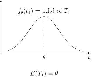 | 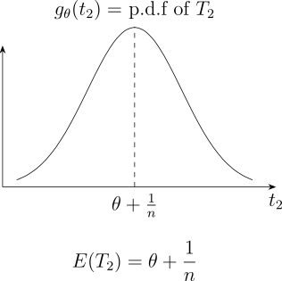 |
\(\var _{\theta }(T_1)\) is large \(\var _{\theta }(T_2)\) is small which estimator is better?
To determine whether a given estimator \(T(X)\) does well for estimating \(\theta \), we consider a loss function or distance between the estimator and the true value denoted by \(L\left (\theta \, , \, T(X)\right )\). This loss function is averaged over all possible values of the data to obtain the risk \[Risk = E_{\theta }\big \{L(\theta \, , \, T(X)\big \}\] A good estimator is one with small risk. One particular loss function is \[L\left (\theta \, , \, T(X)\right ) = \left (T(X) - \theta \right )^2\] which is called the squared error loss function whose corresponding risk, called mean squared error (MSE) is given by \[\MSE _{\theta }(T) = E_{\theta }\left [(T(X) - \theta )^2\right ]\] Another loss function is \[L\left (\theta \, , \, T(X)\right ) = \begin {vmatrix} T(X) - \theta \\ \end {vmatrix}\] which is called the absolute error loss function whose corresponding risk, called the mean absolute error, is given by \[Risk = R\left (\theta \, , \,T\right ) = E_{\theta }\begin {vmatrix} T(X) - \theta \\ \end {vmatrix}\]
Problem 1.2.4. Show that \(\,\, \MSE _{\theta } (T) = \var _{\theta }(T) + \left (\bias _{\theta }(T)\right )^2\,\) where \(\bias _{\theta }(T) = E_{\theta }\left (T(X) - \theta \right )\).
Show solution
Solution. Write \(\mu _T = E_{\theta }\left (T\right )\) and add and subtract it inside the square: \begin {align*} \MSE _{\theta }(T) &= E_{\theta }\left [\left (T-\theta \right )^{2}\right ] = E_{\theta }\left [\left \{\left (T-\mu _T\right ) + \left (\mu _T-\theta \right )\right \}^{2}\right ]\\ &= E_{\theta }\left [\left (T-\mu _T\right )^{2}\right ] + 2\left (\mu _T-\theta \right )E_{\theta }\left [T-\mu _T\right ] + \left (\mu _T-\theta \right )^{2}. \end {align*}
The middle term vanishes because \(E_{\theta }\left [T-\mu _T\right ]=0\), and \(\mu _T-\theta \) is a constant that may be taken outside the expectation. The first term is \(\var _{\theta }(T)\) and the last is \(\left [\bias _{\theta }(T)\right ]^{2}\), giving \[\MSE _{\theta }(T) = \var _{\theta }(T) + \left [\bias _{\theta }(T)\right ]^{2}.\]
Note. The decomposition is the reason unbiasedness is a convenience rather than a virtue. Setting the bias to zero removes one term, but nothing guarantees the sum is smallest there — and the next two problems produce estimators that are biased and beat the unbiased ones outright.
Example 1.2.7. Let \(\, X_1\, , \,X_2\, , \, \cdots \cdots \, X_n\,\) be a random sample from a UNIF\((0,\theta )\) distribution. Compute the MSE’s of the following three estimators of \(\theta \): \[T_1 = 2\overline {X}\hspace {0.4cm},\hspace {0.4cm} T_2 = X_{(n)}\hspace {0.4cm},\hspace {0.4cm} T_3 = (n + 1)X_{(1)}\] where \(X_{(n)} = \max (X_1\, , \, X_2\, \cdots \cdots \, X_n)\) and \(X_{(1)} = \min (X_1\, , \, X_2\, \cdots \cdots \, X_n)\)
Solution. \(\MSE (T_1) = \var (T_1) + (\bias (T_1))^2\) \begin {align*} bias (T_1) & = E(T_1) - \theta \\ & = E\left (2\overline {X}\right ) - \theta = 2\, E(\overline {X}) - \theta \\ & = 2E(X) - \theta \\ & = 2\left (\frac {\theta }{2}\right ) - \theta = 0. \end {align*}
\begin {align*} \MSE (T_1) & = \var (T_1) = \var (2\overline {X})\\ & = 4\, \var (\overline {X}) = \frac {4}{n}\, \var (X)\\ & = \frac {4}{n}\, \frac {\theta ^2}{12}\\ & = \frac {\theta ^2}{3n}. \end {align*}
\(\MSE (T_2) = \var (X_{(n)}) + (\bias (X_{(n)})^2\)
\(Bias(X_{(n)}) = E(X_{(n)}) - \theta \)
Let \(Y = X_{(n)}\) \begin {align*} F(y) & = P(Y\leq y) = P(X_{(n)} \leq y)\\ & = P(X_1\leq y\, , \, X_2\leq y\, , \,\cdots \cdots \, ,\, X_n \leq y)\\ & = \left [F_X(y)\right ]^n \end {align*}
\[f(y) = n\, \left [F_X(y)\right ]^{n-1}\, f_X(y)\]
\begin {align*} \text {So}\hspace {0.8cm}F_X(y) & = P(X\leq x) = \int _0^x\dfrac {1}{\theta }\, \, dt = \dfrac {t}{\theta }\Bigg |_0^x = \dfrac {x}{\theta } \end {align*}
\[f(y) = n\left (\frac {y}{\theta }\right )^{n-1}\, \dfrac {1}{\theta } = \frac {n\, y^{n-1}}{\theta ^n}\hspace {0.5cm}, \hspace {0.3cm} 0 < y < \theta \]
\begin {align*} E\left (X_{(n)}\right ) & = E(Y) = \int _0^{\theta } \frac {y\, n\, y^{n-1}}{\theta ^n}\, dy = \frac {n\theta }{n + 1}. \end {align*}
\[Bias(T_2) = \frac {n\theta }{n+ 1} - \theta = -\frac {\theta }{n + 1}\]
\[\var (T_2) = E\left (T^2_2\right ) - \left (E(T_2)\right )^2\]
\begin {align*} E\left (T_2^2\right ) = E(Y^2) = \int ^{\theta }_0y^2\, \frac {n y^{n-1}}{\theta ^n}\, dy = \frac {n\, \theta ^2}{n + 2}. \end {align*}
\[\var (T_2) = \frac {n\, \theta ^2}{n+2} - \left (\frac {n\, \theta }{n + 1}\right )^2 = \frac {n\, \theta ^2}{(n + 1)^2\, (n + 2)}.\]
\begin {align*} \MSE (T_2) & = \frac {n\, \theta ^2}{(n + 1)^2\, (n + 2)} + \frac {\theta ^2}{(n + 1)^2} = \frac {2\,\theta ^2}{(n + 1)\, (n+ 2)}. \end {align*}
\[\MSE (T_3) = \var (T_3) + \left (\bias (T_3)\right )^2\]
\begin {align*} \bias (T_3) & = E(T_3) - \theta \, = \,E\left ((n + 1)\,X_{(1)}\right ) - \theta \, = \, (n+1)\, E(X_{(1)}) - \theta . \end {align*}
Let \(Y = X_{(1)}\), then \begin {align*} F(y) & = P\left (X_{(1)}\leq y\right )\\\\ & = 1 - P\left (X_{(1)} > y\right )\\\\ & = 1 - P\left (X_1 > y\, , \, X_2>y\, , \, \cdots \cdots \, , \, X_n>y\right )\\\\ & = 1 - \left (1 - F_X(y)\right )^n \end {align*}
\begin {align*} f(y) & = n\, \left (1 - F_X(y)\right )^n\, f_X(y)\\\\ & = n \, \left (1 - \frac {y}{\theta }\right )^{n-1}\, \frac {1}{\theta }\\\\ & = \frac {n}{\theta }\left (1 - \frac {y}{\theta }\right )^{n-1}\hspace {0.5cm},\hspace {0.3cm} 0 < y < \theta \end {align*}
\begin {align*} E\left (X_{(1)}\right ) & = \int _0^{\theta }y\, \frac {n}{\theta }\, \left (1 - \frac {y}{\theta }\right )^{n-1}\, dy\\\\ &\hspace {0.6cm}\text {Let}\hspace {0.3cm} u = 1 - \frac {y}{\theta }\\\\ & = \frac {\theta }{n + 1}. \end {align*}
\begin {align*} E(T_3) & = (n + 1)\, E\left (X_{(1)}\right )\, = \, (n + 1)\, \frac {\theta }{n + 1} = \theta . \end {align*}
\begin {align*} \MSE (T_3) & = \var (T_3)\\\\ & = \var \left [(n+1)\, \left (X_{(1)}\right )\right ]\\\\ & = (n+1)^2\, \var \left (X_{(1)}\right ) \end {align*}
\[\var \left (X_{(1)}\right ) = E\left (X_{(1)}^2\right ) - \left (E(X_{(1)})\right )^2\]
\begin {align*} E\left (X_{(1)}^2\right ) & = E\left (Y^2\right )\, =\, \int _0^{\theta } y^2\, \frac {n}{\theta }\, \left (1 - \frac {y}{\theta }\right )^{n-1}\, dy\, = \,\frac {2\, \theta ^2}{(n + 1)\, (n + 2)}. \end {align*}
\[\var \left (X_{(1)}\right ) = \frac {2\, \theta ^2}{(n + 1)\, (n + 2)} - \frac {\theta ^2}{(n + 1)^2}\, = \, \frac {n\, \theta ^2}{(n + 1)^2 \, (n + 2)}\]
\[MST(T_3) = (n + 1)^2\, \frac {n\, \theta ^2}{(n + 1)^2\, (n + 2)} = \frac {n\, \theta ^2}{n+ 2}\]
i.e \(\, \, T_2\) is the best estimator. □
Problem 1.2.5. Let \(\, X_1\, , \, X_2\, , \, \cdots \cdots \, , \, X_n\,\) be a random sample from a UNIF\((0\, , \, \theta )\) distribution. Consider the following estimators of \(\theta \): \begin {align*} T & = X_{(1)} + X_{(n)}\\ R & = X_{(n)} - X_{(1)} \end {align*}
which estimator is unbiased? Compare the MSE’s of these estimators.
Show solution
Solution. For a sample from UNIF\((0,\theta )\) the extreme order statistics satisfy \[E\left (X_{(1)}\right ) = \frac {\theta }{n+1},\qquad E\left (X_{(n)}\right ) = \frac {n\theta }{n+1},\] \[\var \left (X_{(1)}\right ) = \var \left (X_{(n)}\right ) = \frac {n\theta ^{2}}{(n+1)^{2}(n+2)}, \qquad \cov \left (X_{(1)},X_{(n)}\right ) = \frac {\theta ^{2}}{(n+1)^{2}(n+2)} .\]
Which is unbiased
\[E(T) = \frac {\theta }{n+1} + \frac {n\theta }{n+1} = \theta ,\qquad E(R) = \frac {n\theta }{n+1} - \frac {\theta }{n+1} = \frac {(n-1)\theta }{n+1}.\] So \(T\) is unbiased and \(R\) is not; \(R\) has bias \(-2\theta /(n+1)\), which is negative because the range of a sample can never reach the full length \(\theta \).
Comparing mean square errors
Adding the variances with the covariance term, \[\var (T) = 2\var \left (X_{(1)}\right ) + 2\cov \left (X_{(1)},X_{(n)}\right ) = \frac {2\theta ^{2}}{(n+1)(n+2)},\] \[\var (R) = 2\var \left (X_{(1)}\right ) - 2\cov \left (X_{(1)},X_{(n)}\right ) = \frac {2(n-1)\theta ^{2}}{(n+1)^{2}(n+2)} .\] Since \(T\) is unbiased, \(\MSE (T) = \var (T)\). For \(R\), adding the squared bias, \[\MSE (R) = \frac {2(n-1)\theta ^{2}}{(n+1)^{2}(n+2)} + \frac {4\theta ^{2}}{(n+1)^{2}} = \frac {6\theta ^{2}}{(n+1)(n+2)} .\] Therefore \[\frac {\MSE (R)}{\MSE (T)} = 3 \qquad \text {for every } n .\] \(T\) beats \(R\) by a factor of three at every sample size. The ratio does not depend on \(n\) or on \(\theta \), so no sample size rescues \(R\).
Problem 1.2.6. Let \(\, X_1\, , \, X_2\, , \, \cdots \cdots \, , \, X_n\,\) be a random sample from the \(N(\mu \, , \, \sigma ^2)\) distribution. Consider the following estimators of \(\sigma ^2\): \[T_1= \frac {n - 1}{n}S^2\hspace {0.8cm}, \hspace {0.8cm} T_2 = \frac {n - 1}{n + 1}\, S^2\hspace {0.8cm}\text {where}\hspace {0.5cm}S^2 = \frac {1}{n - 1}\sum ^n_{i = 1}\left (X_i - \overline {X}\right )^2\] Compare the MSE’s of these estimators by grouping them as a function of \(\sigma ^2\) for \(n = 5\).
Show solution
Solution. Under normality \(W = (n-1)S^{2}/\sigma ^{2} \sim \chi ^{2}_{(n-1)}\), so \(E(W)=n-1\) and \(\var (W)=2(n-1)\). Both estimators have the form \(c\,\sigma ^{2}W\): for \(T_1\), \(c=1/n\); for \(T_2\), \(c=1/(n+1)\). For such an estimator \[\MSE = c^{2}\sigma ^{4}\var (W) + \left [c\,\sigma ^{2}E(W) - \sigma ^{2}\right ]^{2} = \sigma ^{4}\left \{2(n-1)c^{2} + \left [c(n-1)-1\right ]^{2}\right \}.\] Substituting the two values of \(c\), \[\MSE (T_1) = \frac {(2n-1)\,\sigma ^{4}}{n^{2}},\qquad \MSE (T_2) = \frac {2\,\sigma ^{4}}{n+1} .\] For comparison the unbiased \(S^{2}\) itself has \(\MSE (S^{2}) = 2\sigma ^{4}/(n-1)\).
At \(n=5\)
\[\MSE (T_1) = \frac {9}{25}\sigma ^{4} = 0.360\,\sigma ^{4},\qquad \MSE (T_2) = \frac {1}{3}\sigma ^{4} \approx 0.333\,\sigma ^{4},\qquad \MSE (S^{2}) = \frac {1}{2}\sigma ^{4} .\] The ordering is \(\MSE (T_2) < \MSE (T_1) < \MSE (S^{2})\), and it holds for every \(n\), not only \(n=5\).
Remark. Minimising \(2(n-1)c^{2} + \left [c(n-1)-1\right ]^{2}\) over \(c\) gives \(c = 1/(n+1)\) exactly, so \(T_2\) is not merely better than the other two — it is the best estimator of the form \(cS^{2}\) there is. The unbiased choice \(c=1/(n-1)\) is the worst of the three. This is the clearest illustration in the chapter of the point made in the previous problem: insisting on unbiasedness costs accuracy.
Example 1.2.8. Let \(\, X\thicksim N(\theta \, ,\, 1)\). Compare the MSE’s of the three estimators \[T_1 = X\hspace {0.8cm}, \hspace {0.8cm} T_2 = \frac {X}{2}\hspace {0.8cm},\hspace {0.8cm} T_3 = 0\]
Solution. \(\MSE (T_1) = \var (T_1) + \left (\bias (T_1)\right )^2\)
\(E(T_1) = E(X) = \theta \hspace {0.8cm}\) unbiased.
\[\MSE (T_1) = \var (T_1) = \var (X) = 1.\]
\(\MSE (T_2) = \var (T_2) + \left (\bias (T_2)\right )^2\)
\(E(T_2) = \frac {\theta }{2}\,\) and \(\, \var (T_2) = \frac {1}{4}\)
\begin {align*} \bias (T_2) & = E(T_2) - \theta = \frac {\theta }{2} - \theta \,= -\,\frac {\theta }{2} \end {align*}
\[\MSE (T_2) = \dfrac {1}{4} + \dfrac {\theta ^2}{4}\]
\(\MSE (T_3) = \var (T_3) + \left (\bias (T_3)\right )^2\)
We have that \(\,E(T_3) = 0\) and \(\var (T_3) = 0\) which implies that \(\bias (T_3) = E(T_3) - \theta = -\theta \)
\[\MSE (T_3) = \theta ^2\]
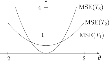
i.e \(\, \) No estimator outperforms all other estimators even the trivial estimator \(T_3\) is better for some
values of \(\theta \).
In order to achieve a best estimator, we need to restrict ourselves to a specific class of estimators
and select the best within the class. One possible restriction is to the class of unbiased
estimators. □
1.2.2 Uniformly Minimum Variance Unbiased Estimation
Definition 1.2.9. An estimator \(T(X)\) is said to be uniformly minimum variance unbiased estimator \((UMVUE)\) of the parameter \(\theta \) if
- i.
- it is an unbiased estimator of \(\theta \)
- ii.
- among all unbiased estimators of \(\theta \) it has the smallest \(MSE\) and therefore the smallest variance.
Questions on this section
Stuck on something here? Ask below and it stays attached to this topic.