3.4 Choosing a model

The exponential is the Weibull with \(k = 1\), so the two can be compared by a likelihood ratio test: \(2(\ell _{\text {Weibull}} - \ell _{\text {exp}})\) is approximately \(\chi ^2_1\) if \(k = 1\). Non-nested families are compared by the Akaike information criterion \(\text {AIC} = -2\ell + 2p\), with \(p\) the number of parameters; smaller is better. Graphical checks are also useful: for the Weibull, \(\log H(t) = k\log t - k\log \lambda \), so a plot of \(\log (-\log \hat S(t))\) against \(\log t\) from a non-parametric estimate \(\hat S\) should be close to a straight line with slope \(k\); the next section supplies such an estimate.

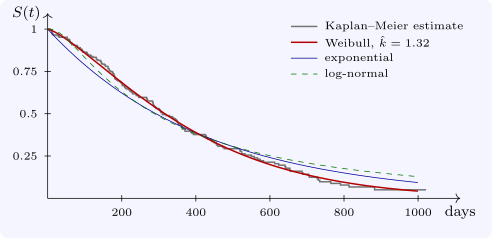
Example 3.4.1. For lung, the maximised log-likelihoods are \(-1162.3\) (exponential), \(-1153.9\) (Weibull), \(-1169.3\) (log-normal) and \(-1160.9\) (log-logistic). The Weibull has the smallest AIC, \(2311.7\). Its shape is \(\hat k = 1.32\), an increasing hazard, and the likelihood ratio statistic against the exponential is \(17.0\) on one degree of freedom, \(p = 0.00004\): the death rate rises with time since enrolment. The fitted Weibull median is \(316\) days, longer than the exponential’s \(292\) (Figure 3).

dS20406080100.0.0.1KWexloay(t00000257apepgs)055libo-nanuneor–ll,nmM ˆktiae=allier1es.3ti2mate — Figure 3: Parametric fits to the lung data, with the non-parametric Kaplan–Meier estimate of the next section as a reference. The Weibull follows the data closely; the exponential is too low early and too high late, because the true hazard increases; the log-normal, whose hazard eventually falls, has too heavy a tail.

[next] [prev] [prev-tail] [front] [up]

Questions on this section

Stuck on something here? Ask below and it stays attached to this topic.