2.1 Random Variables
Definition 2.1.1. A random variable denoted by \(X\) is a function whose value is a real number determined by each element in the sample space. \[X:S\longrightarrow \mathbb {R}\] \(S\) is the domain of \(X\), \(\, \mathbb {R}_X\) is the range (space of the random variable \(X\)) which is the subset of \(\mathbb {R}\).
Note 2.1.2. A random variable is neither random nor variable, it is simply a function. The values it takes on are both random and variable.
Example 2.1.3. Consider tossing a fair coin three times. The sample space \(S\) contains 8 outcomes. If we define \(X\) as the number of heads, the random variable maps each sequence to an integer:
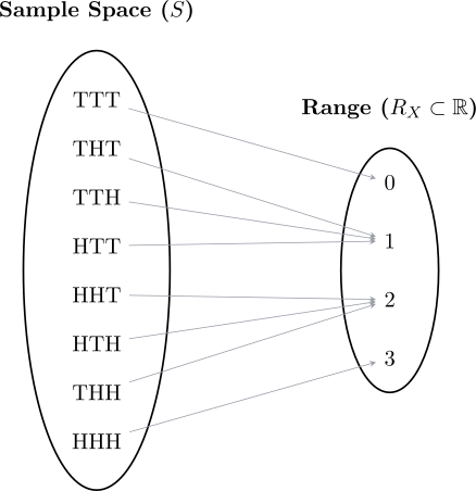
Example 2.1.4. In industrial monitoring, such as that performed by the Environmental Council of Zambia (ECZ), the nature of the data determines the classification of the variable.
- 1.
- Pesticide Concentration (\(X\)): if we measure the mass of pesticide in milligrams per liter, \(X\) can take any value in a continuous interval. Then the range is \[R_X = \{x \in \mathbb {R} : x \geq 0\},\] and the data type is continuous (uncountably infinite outcomes).
- 2.
- Monthly Compliance (\(X\)): if we count the number of months until a company fails an inspection, \(X\) can be any whole number. The range is \[R_X = \{0, 1, 2, 3, \dots \},\] and the data type is discrete (countably infinite outcomes).
Note 2.1.5. In practice, we use \(X\) (uppercase) to refer to the name of the variable and \(x\) (lowercase) to refer to a specific value it might take.
2.1.1 Summation methods you will need
Four standard series account for almost every sum in this course. They are collected here because the algebra of a distribution is usually harder than its probability: showing that a probability function sums to 1, or deriving a moment generating function, nearly always comes down to recognising one of these four.
Technique 2.1.1 (Geometric series). For \(|r|<1\), \[a+ar+ar^{2}+\cdots = \frac {a}{1-r}, \qquad \text {in particular}\qquad \sum _{k=0}^{\infty }r^{k} = \frac {1}{1-r}.\] The finite version needs no condition on \(r\): \[a+ar+\cdots +ar^{n} = \frac {a\left (1-r^{n+1}\right )}{1-r}, \qquad r\neq 1.\]
Take care where the sum starts. A series beginning at \(k=1\) is missing the term \(k=0\), so \[\sum _{k=1}^{\infty }r^{k} = \frac {1}{1-r}-1 = \frac {r}{1-r}.\] This one detail causes more lost marks than any other in the topic. You will use the geometric series to normalise the geometric distribution and to find its m.g.f.
Technique 2.1.2 (Binomial theorem). For a positive integer \(n\), \[(1+x)^{n} = \sum _{k=0}^{n}\binom {n}{k}x^{k}.\] When \(n\) is not a positive integer the sum becomes infinite and needs \(|x|<1\): \[(1+x)^{n} = \sum _{k=0}^{\infty }\binom {n}{k}x^{k}, \qquad |x|<1,\] where \(\dbinom {n}{k} = \frac {n(n-1)\cdots (n-k+1)}{k!}\) for any real \(n\).
The second form is the one that matters here: with a negative upper index it gives the negative binomial distribution its name and its moment generating function.
Technique 2.1.3 (Vandermonde’s identity). For non-negative integers \(a\), \(b\), \(n\), \[\sum _{x}\binom {a}{x}\binom {b}{n-x} = \binom {a+b}{n}.\]
The sum may be written as running to infinity, but it is really finite: \(\binom {a}{x} = 0\) as soon as \(x>a\), since one cannot choose more objects than exist. For example \(\binom {4}{5} = 0\).
There is a direct way to see why it is true. To choose \(n\) objects from \(a+b\), split the \(a+b\) into a group of \(a\) and a group of \(b\). Any selection takes some number \(x\) from the first group and the remaining \(n-x\) from the second; summing over every possible \(x\) counts each selection exactly once. This identity is what makes the hypergeometric probabilities sum to 1. (It appears again as Remark 1.5.8.)
Technique 2.1.4 (Exponential series). For every real \(x\), \[e^{x} = 1+x+\frac {x^{2}}{2!}+\frac {x^{3}}{3!}+\cdots = \sum _{k=0}^{\infty }\frac {x^{k}}{k!}.\]
This is what makes the Poisson probabilities sum to 1, and it is the series that appears whenever a moment generating function is expanded to read off moments.
Solution. \[\sum _{x=0}^{\infty }\frac {\lambda ^{x}e^{-\lambda }}{x!} = e^{-\lambda }\sum _{x=0}^{\infty }\frac {\lambda ^{x}}{x!} = e^{-\lambda }\cdot e^{\lambda } = 1,\] using the exponential series with \(x = \lambda \). Recognising which series applies is the whole of the work; the rest is cancellation.
2.1.2 Practice Problems
Problem 2.1.1. For each of the following random variables write the possible values, and hence classify them as discrete or continuous.
- (a).
- The number of automobile accidents each year in Lusaka.
- (b).
- The amount of milk produced yearly by a particular cow.
- (c).
- The number of eggs laid each month by one hen.
- (d).
- The number of building permits issued each month in Lusaka.
- (e).
- The weight of maize grain in kilograms produced per acre.
Show solution
Solution. The test is not whether the numbers are large, but whether the possible values can be listed. A variable whose values can be put in a list – even an endless one – is discrete; one that can take any value in an interval is continuous.
- (a).
- \(\{0,1,2,3,\ldots \}\) – a count, so discrete.
- (b).
- Any value in \([0,\infty )\) – continuous. In practice it is recorded to the nearest litre, but the quantity itself varies continuously; rounding a measurement does not make the variable discrete.
- (c).
- \(\{0,1,2,\ldots \}\) – a count, discrete.
- (d).
- \(\{0,1,2,\ldots \}\) – a count, discrete.
- (e).
- Any value in \([0,\infty )\) – continuous.
The three discrete ones are all counts of events, and the two continuous ones are both measurements of amount. That is the usual dividing line: counting gives a discrete variable, measuring gives a continuous one.
Questions on this section
Stuck on something here? Ask below and it stays attached to this topic.