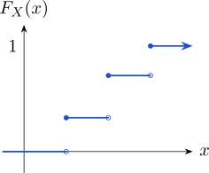
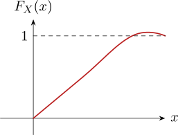
2.7 Cumulative Distribution Function (CDF)

Definition 2.7.1. Let \(X\) be a random variable with probability function \(f_X(x)\), then cumulative distribution function (cdf) of \(X\) denoted by \(F_X(x)\) and is given by \[F_X(t)=P(X\leq t)\] specifically, calculated as \[F_X(t)= \begin {cases} \sum \limits _{\{X:X\leq t\}}P(X=x) & \text {if}\quad X \quad \text {discrete}\\ \displaystyle {\int \limits _{\{X:X\leq t\}}}f_X(x)\, dx & \text {if}\quad X \quad \text {is continuous}\\ \end {cases} \]

Fundamental Properties:

1.: \(F_X(x)\) is a non-decreasing function.
2.: \(F_X(-\infty ) = \lim _{x \to -\infty } F_X(x) = 0\).
3.: \(F_X(+\infty ) = \lim _{x \to +\infty } F_X(x) = 1\).
4.: \(F_X(x)\) is right-continuous: \(\lim _{h \to 0^+} F_X(x+h) = F_X(x)\).

Example 2.7.2. Consider tossing a fair coin 3 times. Let \(X \sim \operatorname {BIN}(3, 1/2)\).The p.m.f. is: \[f_X(x) = \binom {3}{x} \left (\frac {1}{2}\right )^3\quad \text {for} \quad x \in \{0, 1, 2, 3\}.\] \[P(X = 0) = \frac {1}{8}\, ,\quad P(X = 1) = \frac {3}{8}\, ,\quad P(X = 2) = \frac {3}{8}\, , \quad P(X = 3) = \frac {1}{8}.\] \(F_X(t)=P(X\leq t)\)

If \(\, t < 0\) \[F_X(t)=P(X\leq t)=0.\] If \(\, 0\leq t<1\) \[F_X(t)=P(X\leq t)=P(X\leq 0)=P(X=0)=\frac {1}{8}.\] If \(\, 1 \leq t < 2\) \begin {align*} P(1\leq t< 2) & = P(X\leq 1)=P(X=0,X=1)\\ & = P(X=0)+P(X=1)\\ & = \frac {1}{8}+\frac {3}{8}\\ & = \frac {1}{2}. \end {align*}

If \(\, 2 \leq t < 3\) \begin {align*} P(2 \leq t < 3) & = P(X\leq 2)\\ & = P(X = 0) + P(X = 1) + P(X = 2)\\ & = \frac {1}{8}+\frac {3}{8}+\frac {3}{8}\\ & =\frac {7}{8}. \end {align*}

If \(\, t\geq 3,\) \(\,P(X\leq 3)=1\) since \[P(X=0)+P(X=1)+P(X=2)+P(X=3)=1.\] Therefore, the c.d.f \[F_X(t)= \begin {cases} 0 & \text {if}\hspace {0.3cm}t<0\\\\ \frac {1}{8} & \text {if}\hspace {0.3cm} 0\leq t<1\\\\ \frac {1}{2} & \text {if}\hspace {0.3cm} 1\leq t<2\\\\ \frac {7}{8} & \text {if}\hspace {0.3cm} 2\leq t<3\\\\ 1 & \text {if} \hspace {0.3cm} t\geq 3\\ \end {cases} \] The plot

tF14711234X∕∕∕888(t) — Figure 2.25: Graph of \(F_X(t)\)

Example 2.7.3. Let the pdf of a random variable \(X\) be \[f_X(x)=\frac {x+1}{8},\quad 2<x<4.\] Find the c.d.f and plot it.

Solution. \[F_X(t)=P(X\leq t)=\displaystyle {\int \limits _{\{X:X\leq t\}}}f_X(x)dx\]

If \(\, t \leq 2\), \[F_X(t)=0.\]

If \(t\) is such \(2<t<4\) \begin {align*} F_X(t)=P(X\leq t) & = \int ^t_2f_X(x)\, dx\\ & =\int ^t_2\frac {x+1}{8}dx\\ & = \frac {(x+1)^2}{8}\Big |^t_2\\ & = \frac {(t+1)^2-9}{16}. \end {align*}

If \(\, t\geq 4\), \begin {align*} F_X(t) & = P(X\leq t)\\ & = \int ^t_2f_X(x)\, dx+\int ^t_4f_X(x)\,dx\\ & = 1+0\\ & = 1. \end {align*}

Therefore the c.d.f \[F_X(t)= \begin {cases} 0 & \text {if}\hspace {0.5cm} t\leq 2\\ \frac {(t+1)^2-9}{16} & \text {if}\hspace {0.5cm} 2<t<4\\ 1 & t\geq 4\\ \end {cases} \]

The plot

□

Remark 2.7.4.

1.

In the case where \(X\) is discrete with possible values \(x_1,x_2,x_3,\cdots \) \[f_X(x_j)=P(X=x_j)=F_X(x_j)-F_X(x_{j-1})\]

For continuous random variable \begin {align*} P(a<X<b)& = \int ^a_bf_X(x)dx\\ & = \int ^b_{-\infty }f_X(x)dx-\int ^a_{-\infty }f_X(x)dx\\ & = F_X(b)-F_X(a) \end {align*}

also, \(P(a\leq X< b)=P(a\leq X\leq b)=P(a<X\leq b)\)

2.

From fundamental theorem of calculus, it follows that if \(F_X(t)\) is differentiable then \[f_X(x)=\frac {d}{dx}F_X(x).\]

3.

For discrete random variables \(X\) with possible values in ascending order \(x_1,x_2,x_3,\cdots \) then \[F_X(t)=P(X\leq t)=\sum \limits ^k_{j=1}P(X=x_j)\] where \(k\) is such that \(x_{k-1}<t\leq x_k\).

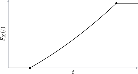
\[F_X(t)= \begin {cases} 0, & t<x_1\\ \sum \limits ^k_{j=1}P(X=x_j) &\\ 1&\text {if}\hspace {0.3cm}t>x_N,\hspace {0.3cm}\text {where}\hspace {0.3cm}x_N\hspace {0.3cm} \text {is the largest}\\ \end {cases} \]

4.

If \(X\) is continuous random variable with pdf having support in the interval \((u,v)\). i.e. \(f_X(x)\) is defined on \((u,v)\) and 0 else where \[ F_X(t)= \begin {cases} 0 & \text {if}\hspace {0.3cm} t<u\\ \displaystyle {\int ^t_uf_X(x)dx} & \text {if}\hspace {0.3cm} u<t<v\\ 1 & \text {if}\hspace {0.3cm} t\geq v\\ \end {cases} \]

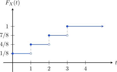
Example 2.7.5. Suppose a random variable has the following probability mass functions: \[P(X = 1) = \frac {1}{2}\, , \quad P(X = 2) = \frac {1}{4}\, ,\quad P(X = 3) = \frac {1}{8}\, , \quad P(X = 4) = \frac {1}{8}.\] Find the c.d.f of the random variable \(X\) and use it to find \(P(X \leq 1)\, , \quad P(1 < X < 3)\) and \(P(1\leq X \leq 3)\).

Solution. The c.d.f \begin {align*} F_X(t) & = \begin {cases} 0, & t < 1\\ \frac {1}{2}, & 1\leq t < 2\\ \frac {3}{4}, & 2\leq t < 3\\ \frac {7}{8}, & 3 \leq < 4\\ 1, & t\geq 4. \end {cases} \end {align*}

The \(P(X\leq 1)\) is \[P(X\leq 1) = F(1^+) = \frac {1}{2}.\] The \(P(1 < X < 3)\) is \begin {align*} P(1 < X < 3) & = F(3^-) - F(1^+)\\ & = \frac {3}{4}-\frac {1}{2}\\ &=\frac {1}{4}. \end {align*}

The \(P(1\leq X \leq 3)\) is \begin {align*} P(1 \leq X \leq 3) & = F(3^+) - F(1^-)\\ & = \frac {7}{8}-0\\ & = \frac {7}{8}. \end {align*} □

Example 2.7.6. Use the c.d.f of \[f_X(x)=\frac {x+1}{8}\, ,\quad 2<x<4\] to find the following probabilities: Using Cdf find:

(i).: \(P(1< X <2\frac {1}{2})\)
(ii).: \(P(2\frac {1}{2}< X \leq 3)\)
(iii).: \(P(3< X <5)\)

Solution. The c.d.f is given by \[F_X(t)= \begin {cases} 0, & t<2\\ \frac {(t+1)^2-9}{16}, & 2\leq t<4\\ 1, & t\geq 4\\ \end {cases} \]

Then \begin {align*} P\left (1<X<2\frac {1}{2}\right ) & =F_X\left (\frac {5}{2}\right )-F_X(1)\\ & = \frac {(2\frac {1}{2}+1)^2-9}{16}-0\\ & = \frac {\frac {49}{4}-9}{16}\\ & = \frac {49-36}{64}\\ & = \frac {13}{64}. \end {align*}

Also \begin {align*} P\left (2\frac {1}{2} < X < 3\right ) & = F_X(3) - F_X\left (\frac {5}{2}\right )\\ & = \frac {(3 + 1)^2 -9}{16}-\frac {13}{64}\\ & = \frac {7}{16}-\frac {13}{64}\\ & =\frac {15}{62}. \end {align*}

And \begin {align*} P(3<X<5) &=F_X(5)-F_X(3)\\ &=1-\left (\frac {4^2-9}{16}\right )\\ & =1-\frac {7}{16}\\ &=\frac {9}{16}. \end {align*} □

Theorem 2.7.7. \(X\thicksim N(\mu ,\sigma ^2)\) is read as \(X\) is distributed as a normal with mean \(\mu \) and variance \(\sigma ^2\). If \[Z=\frac {X-\mu }{\sigma },\] then \(Z\) is distributed as normal with mean 0 and variance 1 and is known as standard normal, notation \(Z\thicksim N(0,1)\).

Note 2.7.8. Normal variable is usually referred to as Gaussian Distribution.

The c.d.f for the standard normal \[\Phi (z)=\int ^z_{-\infty }\frac {e^{\displaystyle {-\frac {1}{2}v^2}}}{\sqrt {2\pi }}\, dv\]

\[\Phi (-1.11)=\int ^{-1.11}_{-\infty }\frac {e^{\displaystyle {-\frac {1}{2}t^2}}}{\sqrt {2\pi }}\, dt\]

−10.11.111 — Figure 2.27: By symmetry, the lower tail below \(z=-1.11\) has the same area as the upper tail above \(z=1.11\); hence \(\Phi (-1.11)=1-\Phi (1.11)\).

\begin {align*} \Phi (-1.11) & = 1-\Phi (1.11)\\ & = 1-0.8643\\ & = 0.1357\\ \end {align*}

\(P(z\geq 2)=P(z>2)\)

Figure 2.28: \(P(Z\geq 2)\) is the area in the upper tail beyond \(z=2\).

\begin {align*} P(z\geq 2) & = 1-P(z\leq 2)\\ & = 1-\Phi (2)\\ & = 1-0.9772\\ & = 0.0228 \end {align*}

\begin {align*} P(-1.02<z<1.96) & = \Phi (1.96)-\Phi (-1.02)\\ & = \Phi (1.96)-(1-\Phi (1.02))\\ & = \Phi (1.96)+\Phi (1.02)-1\\ & = 0.9750+0.8461-1\\ & = 0.8211 \end {align*}

Example 2.7.9. The Rock well hardness of a metal specimen is determined by pressing the surface of the specimen with hardened point, and then measuring the depth of penetration. The hardness of an alloy is normally distributed with mean 70 units and standard deviation 3 units.

1.: If a specimen is acceptable only if its hardness is between 66 and 74 units. What is the probability that a randomly chosen specimen is acceptable?

Solution. \(P(66\leq x\leq 74)= \)? \begin {align*} P\left (\frac {66-70}{3}< Z <\frac {74-70}{3}\right ) & = P\left (-\frac {4}{3}< Z <\frac {4}{3}\right )\\ & = 2P\left (0 < Z <\frac {4}{3}\right )\\ & = 2\left [\Phi \left (\frac {4}{3}\right )-\Phi (0)\right ]\\ & = 2[0.9082-0.5000]\\ & = 0.8164 \end {align*} □
2.: If the acceptable range is \(70\pm c\), for what value of \(c\) would \(95\%\) of all the specimens to be acceptable?

Solution. \[P\left (-\frac {c}{3}< Z <\frac {c}{3}\right ) = 0.95\] \[2P\left (0<z<\frac {c}{3}\right ) = 0.95\] \[\implies P\left (0< Z <\frac {c}{3}\right ) = 0.475\] Therefore \[\frac {c}{3} =1.960\, \, \implies \,\, c=3\times 1.960=5.880\]

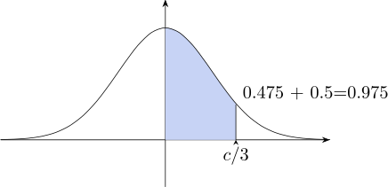
Figure 2.29: \(P(0<Z<c/3)=0.475\), so the area to the left of \(c/3\) is \(0.975\).

□

2.7.1 Practice problems

Problem 2.7.1. [Tutorial Sheet 2] The c.d.f. of a continuous random variable \(X\) is given by \[F(x) = \begin {cases} 0 & x<0\\[2pt] \frac {1}{2}x-\frac {1}{8}x^2 & 0\leq x<1\\[6pt] a+\frac {1}{4}x & 1\leq x<2\\[6pt] b+\frac {1}{8}x^2-\frac {1}{4}x & 2\leq x\leq 3\\[6pt] 1 & x>3. \end {cases}\] Find

(a).: the values of \(a\) and \(b\);
(b).: the p.d.f. of \(X\);
(c).: the mean and standard deviation of \(X\);
(d).: \(P\left (1\leq X<\frac {5}{2}\right )\).

Show solution

Solution. (a). The c.d.f. of a continuous random variable is continuous, so the pieces must agree where they meet. That is what determines \(a\) and \(b\).

At \(x=1\): \[\frac {1}{2}(1)-\frac {1}{8}(1)^2 = a+\frac {1}{4}(1) \implies \frac {3}{8} = a+\frac {1}{4} \implies a = \frac {1}{8}.\] At \(x=2\): \[a+\frac {1}{4}(2) = b+\frac {1}{8}(2)^2-\frac {1}{4}(2) \implies \frac {1}{8}+\frac {1}{2} = b+\frac {1}{2}-\frac {1}{2} \implies b = \frac {5}{8}.\] As a check, the last piece must reach 1 at \(x=3\): \(\tfrac 58+\tfrac 98-\tfrac 34 = 1\). It does.

(b). The density is the derivative of the c.d.f. on each piece: \[f(x) = F'(x) = \begin {cases} \frac {1}{2}-\frac {1}{4}x & 0\leq x<1\\[6pt] \frac {1}{4} & 1\leq x<2\\[6pt] \frac {1}{4}x-\frac {1}{4} & 2\leq x\leq 3\\[6pt] 0 & \text {otherwise.} \end {cases}\] It integrates to 1, as it must.

(c). The density falls from \(\tfrac 12\) to \(\tfrac 14\), is flat, then rises from \(\tfrac 14\) back to \(\tfrac 12\) – it is symmetric about \(x = \tfrac 32\), so \(E(X) = \tfrac 32\). Confirming by integration, \[E(X) = \int _0^1 x\left (\tfrac 12-\tfrac {x}{4}\right )dx + \int _1^2 \frac {x}{4}\,dx + \int _2^3 x\left (\tfrac {x}{4}-\tfrac 14\right )dx = \frac {3}{2}.\] For the variance, \[E(X^2) = \int _0^1 x^2\left (\tfrac 12-\tfrac {x}{4}\right )dx + \int _1^2 \frac {x^2}{4}\,dx + \int _2^3 x^2\left (\tfrac {x}{4}-\tfrac 14\right )dx = \frac {19}{6},\] so \[\operatorname {Var}(X) = \frac {19}{6}-\left (\frac {3}{2}\right )^{2} = \frac {11}{12} \approx 0.917,\] and the standard deviation is \(\sqrt {11/12}\approx 0.957\).

(d). Work directly from the c.d.f.: \[P\left (1\leq X<\tfrac 52\right ) = F\left (\tfrac 52\right )-F(1) = \left (\frac 58+\frac {25}{32}-\frac 58\right )-\frac 38 = \frac {25}{32}-\frac {12}{32} = \frac {13}{32}.\] Because \(X\) is continuous, \(P(X=1) = 0\), so it makes no difference here whether the endpoint is included.

Problem 2.7.2. [Assignment] Derive the cumulative distribution function of each of the following.

(a).: \(f_X(x) = \frac {1}{b-a}\) for \(x\in [a,b]\), and \(0\) otherwise.
(b).: \(f_X(x) = \frac {x-1}{36}\) for \(x = 2,\ldots ,6\) and \(\frac {13-x}{36}\) for \(x = 7,\ldots ,12\).
(c).: \(f_X(x) = \frac {3x^{2}}{7}\) for \(x\in [1,2]\), and \(0\) otherwise.

Show solution

Solution. (a). The uniform distribution. For \(a\leq t\leq b\), \[F(t) = \int _a^{t}\frac {1}{b-a}\,dx = \frac {t-a}{b-a},\] so \[F(t) = \begin {cases} 0 & t<a\\ \frac {t-a}{b-a} & a\leq t\leq b\\ 1 & t>b.\end {cases}\] The c.d.f. rises in a straight line – the defining picture of a uniform distribution.

(b). This is the distribution of the total on two dice. It is discrete, so the c.d.f. is a step function: accumulate the probabilities. Writing everything over 36, the p.m.f. is \(\tfrac {1}{36},\tfrac {2}{36},\ldots ,\tfrac {5}{36}\) for \(x = 2,\ldots ,6\), then \(\tfrac {6}{36}\) at \(x=7\), then back down \(\tfrac {5}{36},\ldots ,\tfrac {1}{36}\). So \(F(t) = \tfrac {1}{36},\tfrac {3}{36},\tfrac {6}{36},\tfrac {10}{36},\tfrac {15}{36}, \tfrac {21}{36},\tfrac {26}{36},\tfrac {30}{36},\tfrac {33}{36},\tfrac {35}{36},1\) on \(2\leq t<3\), \(3\leq t<4\), and so on up to \(t\geq 12\), with \(F(t) = 0\) for \(t<2\).

(c). For \(1\leq t\leq 2\), \[F(t) = \int _1^{t}\frac {3x^{2}}{7}\,dx = \left [\frac {x^{3}}{7}\right ]_1^{t} = \frac {t^{3}-1}{7},\] so \[F(t) = \begin {cases} 0 & t<1\\ \frac {t^{3}-1}{7} & 1\leq t\leq 2\\ 1 & t>2,\end {cases}\] and as a check \(F(2) = \tfrac {8-1}{7} = 1\).

Problem 2.7.3. [Assignment] Given the following cumulative distribution functions, find the corresponding probability functions, and then the stated probabilities.

(a).: \(F_X(t) = 1-e^{-t^{2}/(2\lambda ^{2})}\) for \(t\geq 0\) (and 0 for \(t<0\)), where \(\lambda >0\). Find \(P(\lambda <X<2\lambda )\).
(b).: \(F_X(t) = \frac {t^{2}}{K^{2}}\) for \(0\leq t<K\), with \(F=0\) below and \(F=1\) above, where \(K>0\). Find \(P\left (\frac {K}{3}<X<\frac {K}{2}\right )\).
(c).: \(F_X\) is the step function taking values \(0,\ \frac 14,\ \frac 38,\ \frac 58,\ \frac 34,\ 1\) on \(t<1\), \(1\leq t<3\), \(3\leq t<5\), \(5\leq t<7\), \(7\leq t<9\), \(t\geq 9\). Find \(P(2<X<8)\).

Show solution

Solution. For a continuous variable the density is the derivative of the c.d.f.; for a discrete one the probabilities are the jumps.

(a). Differentiating, \[f_X(t) = \frac {d}{dt}\left (1-e^{-t^{2}/(2\lambda ^{2})}\right ) = \frac {t}{\lambda ^{2}}e^{-t^{2}/(2\lambda ^{2})}, \qquad t\geq 0.\] (This is the Rayleigh distribution.) Then \[P(\lambda <X<2\lambda ) = F(2\lambda )-F(\lambda ) = e^{-1/2}-e^{-2} \approx 0.6065-0.1353 = 0.4712.\]

(b). \[f_X(t) = \frac {2t}{K^{2}}, \qquad 0\leq t<K,\] and \[P\left (\frac {K}{3}<X<\frac {K}{2}\right ) = \frac {(K/2)^{2}}{K^{2}}-\frac {(K/3)^{2}}{K^{2}} = \frac {1}{4}-\frac {1}{9} = \frac {5}{36}.\] Notice the answer does not depend on \(K\) – it is a pure scale parameter.

(c). The jumps occur at \(1,3,5,7,9\) and their sizes are the probabilities: \[P(1) = \tfrac 14,\quad P(3) = \tfrac 18,\quad P(5) = \tfrac 14,\quad P(7) = \tfrac 18,\quad P(9) = \tfrac 14,\] which sum to 1. For the probability, the interval \(2<X<8\) picks up the atoms at \(3, 5\) and \(7\): \[P(2<X<8) = \tfrac 18+\tfrac 14+\tfrac 18 = \frac {1}{2}.\] Equivalently \(F(8)-F(2) = \tfrac 34-\tfrac 14 = \tfrac 12\). With a discrete variable it pays to be careful about whether an endpoint carries an atom; here neither 2 nor 8 does, so strict and non-strict inequalities agree.

[next] [prev] [prev-tail] [front] [up]

Questions on this section

Stuck on something here? Ask below and it stays attached to this topic.