3.3 Conditional Probability Functions and Independence of Random Variables
Definition 3.3.1. Let \(X\) and \(Y\) have a joint probability function \(f_{X,Y}(x,y)\). Then the conditional distribution of \(X\) given \((Y=y^*)\) denoted by \(f_{X/Y}(x/y^*)\) and is given by \[f_{X/Y}(x/y^*)=\frac {f_{X,Y}(x,y^*)}{f_Y(y^*)}\] Thus if \(X\) and \(Y\) are discrete then \[f_{X/Y}(x/y^*)=\frac {f_{X,Y}(x,y^*)}{f_Y(y)}=\frac {P(X=x, Y=y^*)}{P(Y=y^*)}.\] In general \(f_{X,Y}(x,y^*)\) is the joint function evaluated at \(Y=y^*\). \(f_Y(y^*)\) is the marginal probability function of \(Y\) evaluated at \(Y=y^*\).
Similarly the conditional distribution of \(Y\) given \(X=x^*\) given by \[f_{Y/X}(y/x^*)=\frac {f_{X,Y}(x^*,y)}{f_X(x^*)}.\]
Example 3.3.2. Consider the following jointly distributed random variables \(X\) and \(Y\).
| \(Y\) | 0 | 1 | 2 | \(f_Y(y)\) |
| 0 | 0.05 | 0.05 | 0.10 | 0.2 |
| 1 | 0.10 | 0.25 | 0.05 | 0.4 |
| 2 | 0.10 | 0.15 | 0.05 | 0.3 |
| 3 | 0.05 | 0.05 | 0.00 | 0.1 |
| \(f_X(x)\) | 0.30 | 0.50 | 0.20 |
Find the conditional probability mass function of \(Y\) given that \(X = 0\).
Solution. \(f_{Y/X}(y/0)=\) conditional distribution of \(Y\) given \(X=0\) \[f_{Y/X}(y/0)=\frac {f_{X,Y}(y/0)}{f_X(0)}=\frac {P(X=0,Y=y)}{P(X=0)}=\frac {P(X=0,Y=y)}{0.3}.\] We have that \begin {align*} f_{Y/X}(y/0) & = \frac {P(X=0,Y=0)}{0.3}, \quad y = 0\\ & = \frac {P(X=0,Y=1)}{0.3}\, , \quad y = 1\\ & = \frac {P(X=0,Y=2)}{0.3}\, , \quad y = 2\\ & = \frac {P(X=0,Y=3)}{0.3}\, , \quad y = 3. \end {align*}
Therefore
| \(Y\) | 0 | 1 | 2 | 3 | ||
| \(f_{Y/X}(y/0)\) | \(\frac {1}{6}\) | \(\frac {1}{3}\) | \(\frac {1}{3}\) | \(\frac {1}{6}\) |
Example 3.3.3. Suppose that the joint distribution of \(X\) and \(Y\) is given by \[f(x,y) = \begin {cases} \frac {e^{-x/y}\,e^{-y}}{y}\, , & 0 < x < \infty , \quad 0 < y < \infty \\ 0\,, \quad \text {otherwise} \end {cases}.\] Find \(\, P[X > 1/Y = 1].\)
Solution. We first obtain the conditional distribution of \(X\) given that \(Y = y\). \[f{X/Y}(x/y) = \frac {f(x,y)}{f_Y(y)}\] Then marginal \(f_Y(y)\) is \[f_Y(y) = \frac {1}{y}e^{-y}\int ^{\infty }_0 e^{-x/y}\, dx = \frac {1}{y}e^{-y}\left [-ye^{-x/y}\right ]^{\infty }_0 = e^{-y}.\] Hence, \[f_{X/Y}(x/y = 1) = \frac {e^{-x}\, e^{-1}}{e^{-1}} = e^{-x}.\] Therefore \[P[X > 1 / Y = 1] = \int ^{\infty }_1e^{-x}\, dx = \left [-e^{-x}\right ]^{\infty }_1 = e^{-1}.\] □
Definition 3.3.4. Let \(X\) and \(Y\) have a joint probability function \(f_{X,Y}(x,y)\) , \(X\) and \(Y\) are said to be independent if and only if \[f_{X,Y}(x,y)=f_X(x)f_Y(y)\] where \(f_X(x)\) and \(f_Y(y)\) are the marginal probability functions of \(X\) and \(Y\) respectively.
Theorem 3.3.5. If \(X\) and \(Y\) have a joint probability function \(f_{X,Y}(x,y)\) and \(X\) and \(Y\) are independent then \[f_{X/Y}(x/y^*)=f_X(x)\quad \text {and}\quad f_{Y/X}(y/x^*)=f_Y(y).\]
Proof. In the independent case \[f_{X/Y}(x/y^*) = \frac {f_{X,Y}(x,y)}{f_Y(y^*)}=\frac {f_{X,Y}(X=x,Y=y^*)}{f_Y(y^*)} = \frac {f_X(x)\cdot f_Y(y^*)}{f_Y(y^*)} = f_X(x).\] □
Example 3.3.6. For the joint distribution of \(X\) and \(Y\) given by \[f_{X,Y}(x,y)=\frac {\binom {3}{x}\binom {2}{y}\binom {3}{2-x-y}}{\binom {8}{2}}\] the marginals of \(X\) and \(Y\) are \[f_X(x)=\frac {\binom {3}{x}\binom {5}{2-x}}{\binom {8}{2}}\quad x=0,1,2\] and \[f_Y(y)=\frac {\binom {2}{y}\binom {6}{2-y}}{\binom {8}{2}}\quad y=0,1,2\] \(X\) and \(Y\) are not independent because \[f_{X,Y}(x,y)\neq f_X(x) f_Y(y).\]
Exercise 3.3.7. A minibus company receives calls from broken down buses and wrecker crew must haul the buses in for service. The joint distribution of the numbers of calls on Mondays and Tuesdays is given by:
| Tuesdays | 0 | 1 | 2 | 3 | 4 |
| 0 | 0.02 | 0.04 | 0.06 | 0.04 | 0.04 |
| 1 | 0.02 | 0.04 | 0.06 | 0.04 | 0.04 |
| 2 | 0.01 | 0.02 | 0.03 | 0.02 | 0.02 |
| 3 | 0.04 | 0.08 | 0.12 | 0.08 | 0.08 |
| 4 | 0.01 | 0.02 | 0.03 | 0.02 | 0.02 |
Are the number of calls on Mondays and Tuesdays independent?
Theorem 3.3.8. If \(X\) and \(Y\) are independent random variables, \[E(XY) = E(X)\, E(Y)\] provided \(E(X)\) and \(E(Y)\) both exist.
Proof. Suppose that \(X\) and \(Y\) are continuous independent random variables. Then the joint p.d.f can be written as \(f_{X,Y}(x,y) = f_X(x)\, f_Y(y)\). Thus \begin {align*} E(XY) & = \int _x\int _y xy\, f_{X,Y}(x,y)\, dy\, dx\\ & = \int _x\int _y xy\, f_X(x)\, f_Y(y)\, dy \, dx\\ & = \left [\int _x x\, f_X(x)\, dx\right ]\, \left [\int _yy\,f_Y(y)\, dy\right ]\\ & = E(X)\, E(Y). \end {align*} □
Note 3.3.9. When random variables are not independent, a measure of the relationship between them, their covariance, enters into the picture.
Definition 3.3.10. If \(X\) and \(Y\) have a joint distribution function \(f_{X,Y}(x,y)\), then the covariance of \(X\) and \(Y\) denoted by \(Cov(X,Y)\) is given by \[\operatorname {Cov}(X,Y)=E\big \{(X-\mu _X)(Y-\mu _Y)\big \}\] where \(\mu _X=E(X)\) and \(\mu _Y=E(Y)\).
Remark 3.3.11. For the random variables \(X\) and \(Y\):
- 1.
- \(\operatorname {Cov} (X,Y)=E (XY)-E(X)\,(Y)=E(XY)-\mu _X\mu _Y\)
- 2.
- \(\operatorname {Cov} (X,Y)= \operatorname {Cov}(Y,X)\)
- 3.
- \(\operatorname {Cov} (X,X)= \operatorname {Var}(X)\)
- 4.
- Cov\((a\,X,Y) = a\,\)Cov\((X,Y)\)
- 5.
- Covariance is a measure of association.
Definition 3.3.12. If \(X\) and \(Y\) have joint distribution function \(f_{X,Y}(x,y)\) then the correlation coefficient of \(X\) and \(Y\) denoted by \(\rho _{XY}\) and is given by \[\rho _{XY}=\frac {\operatorname {Cov}(X,Y)}{\sqrt {\operatorname {Var}(X)\,\operatorname {Var}(Y)}}.\]
\[\rho _{XY}=\frac {\operatorname {Cov}(X,Y)}{\sqrt {\sigma _X^2\,\sigma _Y^2}}=\frac {\operatorname {Cov}(X,Y)}{\sigma _X\,\sigma _Y}\]
\(\rho _{XY}\) is a standardised measure of association \(-1\leq \rho _{XY}\leq 1\).
Remark 3.3.13. If \(X\) and \(Y\) are independent then, \(\operatorname {Cov}(X,Y)=0\), hence, \(\rho _{XY}=0\). \[\operatorname {Cov}(X,Y) = E(XY) - E(X)\,E(Y) = E(X)\, E(Y) - E(X)\, E(Y) = 0\]
Question. If \(\operatorname {Cov}(X,Y)=0\) does it mean that \(X\) and \(Y\) are independent?
Answer. Yes only if \(X\) and \(Y\) have joint normal distribution. Otherwise no! □
Theorem 3.3.14. The value of the correlation coefficient \(\rho _{XY}\) of \(X\) and \(Y\) is always between \(-1\) and 1. \[-1\leq \rho _{XY} \leq 1\]
Proof. Let \[Q(t)=E\{[(X-\mu _X) + (Y-\mu _Y)t]^2\},\] since \([(X-\mu _X) + (Y-\mu _Y)t]^2\geq 0\) \[\implies E\big \{\big [\big (X-\mu _X\big )+\big (Y-\mu _Y\big )t\big ]^2\big \}\geq 0\] i.e. \(\quad Q(t)\geq 0\) \begin {align*} Q(t) & = E\left \{\left (X-\mu _X\right )^2+2\left (X-\mu _X\right )\left (Y-\mu _Y\right )t+t^2\left (Y-\mu _Y\right )^2\right \}\\ & = E\left (X-\mu _X\right )^2+2E\left [\left (X-\mu _X\right )t\right ]+t^2E\left (Y-\mu _Y\right )^2\\ & = \operatorname {Var}(X)+2\operatorname {Cov}(X,Y)t+t^2\operatorname {Var}(Y). \end {align*}
Therefore \[Q(t)= \operatorname {Var}(Y)t^2+2\operatorname {Cov}(X,Y)t + \operatorname {Var}(X).\] \(Q(t)\) is a quadratic in \(t\), since \(Q(t)\geq 0\) implies its discriminant must be less than or equal to zero.i.e. \[\left [2\operatorname {Cov}(X,Y)\right ]^2-4\operatorname {Var}(Y)\,\operatorname {Var}(X)\leq 0\] \[4\left [\operatorname {Cov}(X,Y)\right ]^2\leq 4\operatorname {Var}(X)\,\operatorname {Var}(Y)\] \[\implies \frac {\left [\operatorname {Cov}(X,Y)\right ]^2}{\operatorname {Var}(X)\,\operatorname {Var}(Y)}\leq 1\] \[\implies \left [\frac {\operatorname {Cov}(X,Y)}{\sqrt {\operatorname {Var}(X)\,\operatorname {Var}(Y)}}\right ]^2\leq 1\] \[\rho ^2_{XY}\leq 1\] Therefore, \(-1\leq \rho _{XY}\leq 1\). □
Example 3.3.15. A random variable \(X\) has a uniform distribution on \([-1,1]\). Let \(Y = X^2\). Find the correlation coefficient between \(X\) and \(Y\).
Solution. Since \(Y = X^2\) \begin {align*} \operatorname {Cov}(X,Y) & = E(XY) - E(X)\, E(X)\\ & = E(X^3) - E(X)\, E(X^2). \end {align*}
Since \(X\) has the probability density function \[f_(x) = \begin {cases} \frac {1}{2}\, & \text {if}\,\, -1\leq x\leq 1,\\ 0 & \text {otherwise},\\ \end {cases}\] we find that \[E(X) = \int ^1_{-1}x, \frac {1}{2}\, dx = 0\] and \[E(X^3) = \int ^1_{-1}x^3\, \frac {1}{2}\, dx = 0.\] Therefore \[\operatorname {Cov}(X,Y) = 0.\] Hence \(\rho = 0\) although \(X\) and \(Y\) are clearly dependent. □
Results of this type complicate the interpretation of \(\rho \) but essentially it is a measure of the degree of linear dependence between \(X\) and \(Y\).
Example 3.3.16. If \(X\) and \(Y\) have joint distribution given on the table.
| \(X\) | ||||
| \(Y\) | 0 | 1 | 2 | \(f_Y(y)\) |
| 0 | \(3/28\) | \(9/28\) | \(3/28\) | \(15/28\) |
| 1 | \(3/14\) | \(3/14\) | 0 | \(12/28\) |
| 2 | \(1/28\) | 0 | 0 | \(1/28\) |
| \(f_X(x)\) | \(10/28\) | \(15/28\) | \(3/28\) | |
Find \(\rho _{XY}\).
Solution. To find \[\rho _{XY}=\frac {\operatorname {Cov}(X,Y)}{\sqrt {\operatorname {Var}(X)\cdot \operatorname {Var}(Y)}},\] we need to find \[\operatorname {Cov}(X,Y)=E(XY)-E(X)\,E(Y),\] \[\operatorname {Var}(X)=E(X^2)-[E(X)]^2\] and \[\operatorname {Var}(Y)=E(Y^2)-[E(Y)]^2.\] The marginals of \(X\) and \(Y\) are
| \(X\) | 0 | 1 | 2 |
| \(f_X(x)\) | \(10/28\) | \(15/28\) | \(3/28\) |
and
| \(Y\) | 0 | 1 | 2 |
| \(f_Y(y)\) | \(15/28\) | \(12/28\) | \(1/28\) |
. Then \[E(X)=\sum ^2_{x=0}\,xf_X(x)\, =\, \frac {15}{28}+\frac {6}{28}=\frac {21}{28}=\frac {3}{4},\]
\[E(X^2)=\sum ^2_{x=0}\, x^2f_X(x)\, =\frac {15}{28}+\frac {12}{28}=\frac {27}{28},\] Hence \[\operatorname {Var}(X)=\frac {27}{28}-\frac {9}{16}=\frac {45}{112}=\frac {9}{4}\cdot \frac {5}{28}.\] Also \[E(Y)=\sum ^2_{y=0}yf_Y(y)\, =\frac {12}{28}+\frac {2}{28}=\frac {14}{28}=\, \frac {1}{2},\]
\[E(Y^2)=\sum ^2_{y=0}y^2f_Y(y)=\frac {12}{28}+\frac {4}{28}=\frac {16}{28}=\,\frac {4}{7}\]
\[\operatorname {Var}(Y)=\frac {4}{7}-\frac {1}{4}=\frac {16-7}{28}=\, \frac {9}{28}.\]
\[E(XY)=1\times \frac {3}{14}=\frac {3}{14}.\] The covariance \[\operatorname {Cov}(X,Y)= \frac {3}{4}-\frac {3}{4}\cdot \frac {1}{2} = \frac {3}{2}\left (\frac {1}{7}-\frac {1}{4}\right ) = \frac {-9}{2\times 28}.\] Therefore \[\rho _{XY} =\frac {\frac {-9}{2\times 28}}{\sqrt {\frac {9}{4}\cdot \frac {5}{28}\cdot \frac {9}{28}}} = \frac {\frac {-9}{2\times 28}}{\frac {9}{28}\cdot \frac {1}{2}\cdot \sqrt {5}} = \frac {-1}{\sqrt {5}}.\] □
Exercise 3.3.17. Suppose that \[f_{XY}(x,y)=\frac {2}{3}(x + 2y)\, , \quad 0 \leq x \leq 1, \quad 0\leq y \leq 1.\] Find \(\rho _{XY}\).
Definition 3.3.18. If \(X\) and \(Y\) have a joint distribution \(f_{XY}(x,y)\) then the conditional expectation is given as follows \[E(X/Y=y^*)= \begin {cases} \sum \limits _Xx\cdot f_{X/Y}\big (x/y^*) & \text {if}\,\, X\,\,\text {is discrete}\\\\ \int \limits _Xx\cdot f_{X/Y}(x/y^*)& \text {if}\,\, X \,\,\text {is continuous}\\ \end {cases} \] where \(f_{X/Y}(x/y^*)\) is the conditional distribution of \(X\) given \(Y=y^*\). \[E(Y/X=x^*)= \begin {cases} \sum \limits _Yy\cdot f_{Y/X}(y/x^*) & \text {if}\,\, Y \,\,\text {is discrete}\\\\ \int \limits _Yy\cdot f_{Y/X}(y/x^*) & \text {if}\,\, Y\,\, \text {is continuous}\\ \end {cases} \]
Example 3.3.19. Consider the following jointly distributed random variables
| \(X\) | 0 | 1 | 2 | \(f_X(x)\) |
| 0 | 0.05 | 0.05 | 0.10 | 0.20 |
| 1 | 0.10 | 0.25 | 0.05 | 0.40 |
| 2 | 0.10 | 0.15 | 0.05 | 0.30 |
| 3 | 0.05 | 0.05 | 0.00 | 0.10 |
| \(f_Y(y)\) | 0.30 | 0.50 | 0.20 |
Find:
- (a).
- \(E(Y/X=1).\)
Solution. The distribution \(f_{Y/X}(y/1)\)
\(Y\) 0 1 2 \(f_{Y/X}(y/1)\) \(0.25\) \(0.625\) \(0.125\) Then the conditional expectation \[E(Y/X=1) = 0\,(0.25) +1\,(0.625) + 2\, (0.125) = 0.875\] □
- (b).
- \(E(X/Y=0)\)
Solution. The distribution \(f_{X/Y}(x/0)\)
\(X\) 0 1 3 3 \(f_{X/Y}(x/0)\) \(0.167\) \(0.333\) \(0.333\) \(0.167\) The conditional expectation \[E(X/Y=0) = 0\, (0.167) +1\, (0.333) + 2\, (0.333) +3\, (0.167) = 1.5\] □
Example 3.3.20. Consider the joint p.d.f of \(X\) and \(Y\) given by \[f_{X,Y}(x,y) = \begin {cases} \frac {12}{5}\,x(2 - x - y) & 0 < x < 1, \quad 0 < y < 1\\ 0 & \text {otherwise}.\\ \end {cases}\] Find \(E(X/Y = 1)\).
Solution. The marginal \begin {align*} f_Y(1) & = \int _0^1\frac {12}{5}x(2-x-1)\, dx\\\ & = \frac {12}{5}\int ^1_0(x - x^2)\, dx\\ & = \frac {12}{5}\left [\frac {x^2}{2}-\frac {x^3}{3}\right ]^1_0\\ & = \frac {12}{5}\left (\frac {1}{6}\right ). \end {align*}
Then we get \[f_{X/Y}(x/1) = \frac {f_{X,Y}(x,1)}{f_Y(1)}= \frac {\frac {12}{5}\, (x-x^2)}{\frac {12}{5}\cdot \frac {1}{6}} = 6(x - x^2).\] Therefore \begin {align*} E[X/Y = 1] & = \int ^1_0x\, f_{X/Y}(x/1)\, dx\\ & = \int ^1_06(x - x^2)\, dx\\ & = 6\left [\frac {x^2}{2} - \frac {x^3}{3}\right ]^1_0\\ & = 6\left [\frac {1}{2}-\frac {1}{3}\right ]\\ & = 1. \end {align*} □
3.3.1 Special Joint Distribution Function (Bivariate Normal)
\(X\) and \(Y\) are said to have the bivariate normal distribution if their joint probability density function is given by
\[f_{X,Y}(x,y)=\frac {1}{\displaystyle {2\pi \sigma _X\sigma _Y\sqrt {1-\rho ^2}}}\, \displaystyle {\exp \bigg \{-\frac {1}{2(1-\rho ^2)}\bigg (\frac {(x-\mu _X)^2}{\sigma ^2_X}-\frac {2\rho (x-\mu _X)(y-\mu _Y)}{\sigma _X\cdot \sigma _Y}+\frac {(y-\mu _Y)^2}{\sigma ^2_Y}\bigg )\bigg \}}\] for \(\,(x,y)\in \mathbb {R}^2, \quad -\infty < x <\infty , \quad -\infty < y < \infty \), and \(\rho = \) correlation coefficient of \(X\) and \(Y\).
\[\mu _X=E\big (X\big ),\hspace {0.5cm}\sigma ^2_X=var\big (X\big )\] \[\mu _Y=E\big (Y\big ),\hspace {0.5cm} \sigma ^2_Y=var\big (Y\big )\]
If \(\rho =0\) \begin {align*} f_{X,Y}(x,y) & = \frac {1}{2\pi \sigma _X\sigma _Y}\exp \bigg \{\displaystyle {-\frac {1}{2}\bigg (\frac {(x-\mu _X)^2}{\sigma ^2_X}+\frac {(y-\mu _Y)^2}{\sigma ^2_Y}\bigg )}\bigg \}\\\\ & = \frac {1}{2\pi \sigma _X\sigma _Y}\exp \bigg \{-\frac {1}{2}\frac {(x-\mu _X)^2}{\sigma ^2_X}\bigg \}\cdot \exp \bigg \{\displaystyle {-\frac {1}{2}\frac {(y-\mu _Y)^2}{\sigma ^2_Y}}\bigg \}\\\\ & = \frac {1}{\sqrt {2\pi \sigma ^2_X}}\exp \bigg \{\displaystyle {-\frac {1}{2}\frac {(x-\mu _X)^2}{\sigma ^2_X}}\bigg \}\cdot \frac {1}{\sqrt {2\pi \sigma ^2_Y}}\exp \bigg \{\displaystyle {-\frac {1}{2}\frac {(y-\mu _Y)^2}{\sigma ^2_Y}}\bigg \}\\\\ & =f_X(x)\cdot f_Y(y) \end {align*}
where \(X\thicksim N\big (\mu _X,\sigma ^2_X\big ),\hspace {0.5cm} Y\thicksim \big (\mu _Y,\sigma ^2_Y\big )\)
\begin {align*} f_X(x) & = \int ^{\infty }_{-\infty }f_{X,Y}(x,y)dy,\hspace {1cm} \text {Let}\hspace {0.4cm} z=\frac {x-\mu _X}{\sigma _X}\\\\ & = \int ^{\infty }_{-\infty }\frac {1}{2\pi \sigma _X\sigma _Y\sqrt {1-\rho ^2}}\exp \bigg \{\displaystyle {-\frac {1}{2(1-\rho ^2)}\bigg (z^2-2\rho z\cdot \frac {(y-\mu _Y}{\sigma _Y}+\frac {(y-\mu _Y)^2}{\sigma ^2_Y}\bigg )}\bigg \}dy \end {align*}
Let \(v=\frac {y-\mu _Y}{\sigma _Y}\hspace {0.5cm} \implies \hspace {0.5cm} dv=\frac {dy}{\sigma _Y}\) 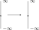
\begin {align*} & = \frac {1}{2\pi \sigma _X}\exp \bigg \{\displaystyle {-\frac {2^2}{2(1-\rho ^2)}}\bigg \}\int ^{\infty }_{-\infty }\frac {1}{\sigma _Y\sqrt {1-\rho ^2}}\exp \bigg \{\displaystyle {-\frac {1}{2}(v^2-2\rho zv)}\bigg \}dv\\\\ & = \frac {1}{2\pi \sigma _X}\int ^{\infty }_{-\infty }\frac {1}{\sqrt {1-\rho ^2}}\exp \bigg \{\displaystyle {-\frac {1}{2(1-\rho ^2)(v^2-2\rho zv+(\rho z)^2-(\rho z)^2}}\bigg \}dv\\\\ &=\frac {\exp \bigg \{\displaystyle {-\frac {z^2}{2(1-\rho ^2)}}\bigg \}\cdot \exp \bigg \{\displaystyle {-\frac {1(\rho ^2z^2)}{2(1-\rho ^2)}}\bigg \}}{2\pi \sigma _X}\int ^{\infty }_{-\infty }\frac {1}{\sqrt {1-\rho ^2}}\exp \bigg \{\displaystyle {-\frac {1}{2(1-\rho ^2)}(v-\rho z)^2}\bigg \}dv\\\\ & =\frac {\exp \bigg \{\displaystyle {-\frac {z^2}{2}}\bigg \}}{\sqrt {2\pi \sigma ^2_X}}\int ^{\infty }_{-\infty }\frac {1}{\sqrt {2\pi (1-\rho ^2)}}\exp \bigg \{\displaystyle {-\frac {1}{2(1-\rho ^2)}(v-\rho z)^2}\bigg \}dv\\ \end {align*}
Let \(w=\frac {v-\rho z}{\sqrt {1-\rho ^2}}\implies dw=\frac {dv}{\sqrt {1-\rho ^2}}\implies \sqrt {1-\rho ^2}dw=dv\)
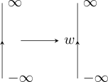
\begin {align*} & = \frac {\exp \bigg \{\displaystyle {-\frac {z^2}{2}}\bigg \}}{\sqrt {2\pi \sigma ^2_X}}\int ^{\infty }_{-\infty }\frac {1}{\sqrt {2\pi }\cdot \sqrt {1-\rho ^2}}\hspace {0.1cm}e^{\displaystyle {-\frac {1}{2}w^2}}\cdot \sqrt {1-\rho ^2}\hspace {0.1cm}dw\\\\ & = \frac {e^{\displaystyle {-\frac {z^2}{2}}}}{\sqrt {2\pi \sigma ^2_X}}\int ^{\infty }_{-\infty }\frac {1}{\sqrt {2\pi }}\hspace {0.1cm}e^{\displaystyle {-\frac {1}{2}w^2}}\hspace {0.1cm}dw\hspace {1cm}\longrightarrow \hspace {0.5cm}\text {the inside is the pdf of N(0,1)}\\\\ & = \frac {e^{\displaystyle {-\frac {z^2}{2}}}}{\sqrt {2\pi \sigma ^2_X}}=\frac {e^{\displaystyle {-\frac {1}{2}\bigg (\frac {x-\mu _X}{\sigma _X}\bigg )}}}{\sqrt {2\pi \sigma ^2_X}}\thicksim N\big (\mu _X,\sigma ^2_X\big ) \end {align*}
It can also be shown that the condition distribution of \(X\) given \(Y=y^*\) is \[N\bigg (\mu _X+\rho \frac {\sigma _X}{\sigma _Y}(y^*-\mu _y),\sigma ^2_X(1-\rho ^2)\bigg )\] , distribution of \(Y\) given \(X=x^*\) is \[N\bigg (\mu _Y+\rho \frac {\sigma _Y}{\sigma _X}(x^*-\mu _X),\sigma ^2_Y(1-\rho ^2)\bigg ).\]
To determine the conditional density of \(X\) given that \(Y = y\), we will continually collect all factors that don not depend on \(x\) and represent them by the constants \(C_i\). \begin {align*} f_{X/Y}(x\vert y) & = \frac {f_{X,Y}(x,y)}{f_Y(y)}\\ & = C1\, f_{X,Y}(x,y)\\ & = C_2 \exp \left \{-\frac {1}{2(1 - \rho ^2)}\left [\left (\frac {x - \mu _X}{\sigma _X}\right )^2 - 2\rho \frac {x(y - \mu _Y)}{\rho _X\rho _Y}\right ]\right \}\\ & = C_3\exp \left \{-\frac {1}{2\sigma ^2_X(1 - \rho ^2)}\left [x^2 - 2x\left (\mu _X + \rho \frac {\sigma _X}{\sigma _Y}(y - \mu _Y\right )\right ]\right \}\\ & = C_4\exp \left \{-\frac {1}{2\sigma ^2_X(1 - \rho ^2)}\left [x - \left (\mu _X + \rho \frac {\sigma _X}{\sigma _Y}(y - \mu _Y\right )\right ]^2\right \} \end {align*}
From the last equation we can conclude that, given \(Y = y\), the random variable \(X\) is normally distributed with mean \(\mu _X + \rho \frac {\sigma _X}{\sigma _Y}(y - \mu _Y)\) and the variance \(\sigma ^2_X(1 - \rho ^2)\).
3.3.2 Practice Problems
Problem 3.3.1. Suppose that \(X\sim \text {BETA}(a,b)\) and \(Y\mid x \sim B(n,x)\). Find (a) \(E(Y)\) and (b) \(\operatorname {Var}(Y)\).
Show solution
Solution. Here the success probability of a binomial is itself random – a mixture. The tools are the tower property and the conditional variance formula: \[E(Y) = E\big [E(Y\mid X)\big ], \qquad \operatorname {Var}(Y) = E\big [\operatorname {Var}(Y\mid X)\big ] + \operatorname {Var}\big [E(Y\mid X)\big ].\] Given \(X=x\), \(Y\) is binomial, so \(E(Y\mid X) = nX\) and \(\operatorname {Var}(Y\mid X) = nX(1-X)\). For the beta distribution, \[E(X) = \frac {a}{a+b}, \qquad \operatorname {Var}(X) = \frac {ab}{(a+b)^{2}(a+b+1)}.\]
(a). \[E(Y) = E(nX) = nE(X) = \frac {na}{a+b}.\]
(b). Take the two pieces in turn. Since \(E(X^{2}) = \operatorname {Var}(X)+\left [E(X)\right ]^{2}\), \[E\big [\operatorname {Var}(Y\mid X)\big ] = n\left [E(X)-E(X^{2})\right ] = n\left [E(X)-E(X)^{2}-\operatorname {Var}(X)\right ],\] \[\operatorname {Var}\big [E(Y\mid X)\big ] = n^{2}\operatorname {Var}(X).\] Adding them and writing \(s = a+b\) for brevity, \begin {align*} \operatorname {Var}(Y) &= n\left [\frac {a}{s}-\frac {a^{2}}{s^{2}}-\frac {ab}{s^{2}(s+1)}\right ] + n^{2}\frac {ab}{s^{2}(s+1)}\\ &= \frac {nab\,(s+n)}{s^{2}(s+1)} = \frac {nab\,(a+b+n)}{(a+b)^{2}(a+b+1)}. \end {align*}
This is the beta–binomial distribution. Compare it with an ordinary binomial having the same mean, whose variance would be \(np(1-p) = \frac {nab}{(a+b)^{2}}\): the mixture carries an extra factor of \(\frac {a+b+n}{a+b+1}\), which exceeds 1 whenever \(n>1\). Letting the success probability vary makes the count more variable than a plain binomial – this is overdispersion, and it is why the beta–binomial is reached for when count data are more scattered than a binomial can explain.
Questions on this section
Stuck on something here? Ask below and it stays attached to this topic.