8 Multicollinearity

The least-squares estimator needs \(\mathbf {X}^\top \mathbf {X}\) to be invertible, which fails exactly when one column of \(\mathbf {X}\) is a linear combination of the others. In practice an exact dependence is rare, but a near dependence is common: one regressor is almost a linear combination of some of the others. This is multicollinearity. It does not violate any assumption of the model, and least squares remains unbiased and best linear unbiased. What it does is make some of the estimates so imprecise that they are of little use, and it does so in ways that the usual output can disguise.

Multicollinearity has four common sources.

(i)

The way the data were collected. If the observations happen to lie close to a line or plane in \(x\)-space, the data cannot separate the effects of the regressors, even if in the population they vary independently. Observational data are especially prone to this.

(ii)

Constraints in the population. Some regressors genuinely move together: household income and house size, or the proportions of the components of a mixture, which must add to \(1\).

(iii)

The choice of model. Polynomial terms such as \(x\) and \(x^2\) are strongly correlated when the range of \(x\) is small compared with its mean.

(iv)

Too many regressors. With more regressors than the data can support, some will inevitably be nearly dependent on the rest.

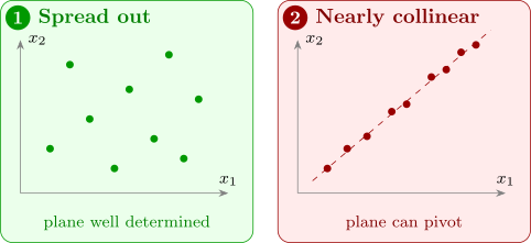
Figure 15 shows why a near dependence matters. To estimate a plane, the data must spread out over the plane’s base. If the points in the \((x_1, x_2)\) plane lie along a line, a whole family of planes, pivoting about that line, fit almost equally well.

Questions on this section

Stuck on something here? Ask below and it stays attached to this topic.