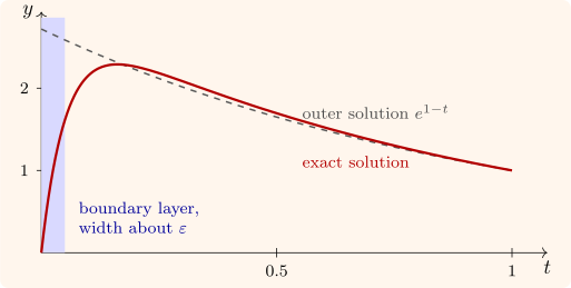
Example 14.4.1. For \(\varepsilon y'' + y' + y = 0\), \(y(0) = 0\), \(y(1) = 1\), with \(0 < \varepsilon \ll 1\), the reduced equation \(y' + y = 0\) is first order, and can satisfy only one condition. The outer solution satisfying \(y(1) = 1\) is \(y_{\text {out}} = e^{1-t}\), which has \(y(0) = e \neq 0\). Near \(t = 0\), in the stretched variable \(\xi = t/\varepsilon \), the equation becomes \(y_{\xi \xi } + y_\xi + \varepsilon y = 0\), with leading-order solution \(y_{\text {in}} = A(1 - e^{-\xi })\); matching \(y_{\text {in}}(\xi \to \infty ) = y_{\text {out}}(0) = e\) gives \(A = e\). The composite approximation, inner plus outer minus their common part, \[ y \approx e^{1-t} - e^{1 - t/\varepsilon } , \] is uniformly accurate to \(O(\varepsilon )\) on \([0, 1]\). The layer has width \(O(\varepsilon )\), and its position is fixed by the sign of the coefficient of \(y'\): with \(-y'\) instead of \(+y'\) the layer would be at \(t = 1\) (Figure 19).