16.3 Discrete-event simulation
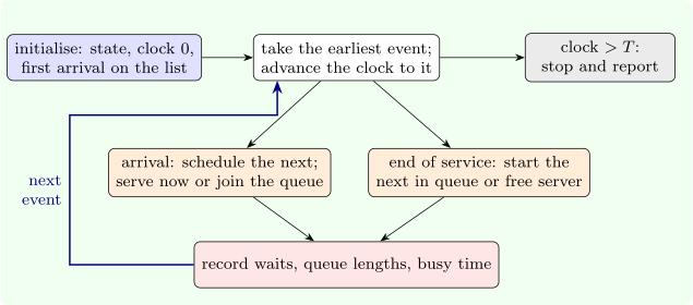
A discrete-event simulation represents a system by its state (the number in each queue, which servers are busy), a clock, and a list of future events ordered by time. The main loop repeatedly removes the earliest event, advances the clock to it, updates the state, schedules the events it causes, and records statistics (Figure 16). For a queue, an arrival schedules the next arrival and either starts a service, scheduling its end, or joins the queue; the end of a service either starts the next customer’s service or frees the server.
Output analysis. The waits of successive customers are strongly correlated, so they cannot be treated as an independent sample. Instead the simulation is run as \(R\) independent replications, each giving one average, and a confidence interval is formed from those \(R\) numbers with the \(t\) distribution; alternatively, one long run is cut into batches whose means are nearly independent. A simulation started empty is biased towards short queues at first, and the warm-up period is discarded. For the bank of Example 14.2.2, \(30\) replications of \(2000\) hours give a mean wait of \(6.42 \pm 0.13\) minutes, covering the exact Erlang C value \(6.47\) (Software 16.5.2): the simulation is verified against a case with a known answer, before it is used for cases without one.
Questions on this section
Stuck on something here? Ask below and it stays attached to this topic.