7.3 The MODI method

The simplex method needs the reduced costs of the non-basic cells. By duality they come from numbers \(u_i\) for the rows and \(v_j\) for the columns, the dual variables of the supply and demand constraints: solve \(u_i + v_j = c_{ij}\) on the \(m + n - 1\) basic cells (with one of them, say \(u_1\), set to \(0\), because of the redundant constraint), and compute \[ d_{ij} = c_{ij} - u_i - v_j \] for the others. If all \(d_{ij} \geq 0\) the solution is optimal. Otherwise the cell with the most negative \(d_{ij}\) enters: adding it to the basic tree creates exactly one cycle, along which the shipments are alternately increased and decreased by \(\theta \); the largest \(\theta \) is the smallest amount on a decreasing cell, which leaves the basis. This is the modified distribution (MODI, or \(u\)–\(v\)) method, the simplex method in the language of the table, with the cycle (the stepping-stone path) playing the role of the ratio test.

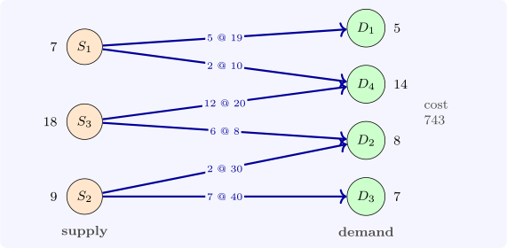
For the VAM solution of Example 7.1.2 the cell \((S_2, D_2)\) has \(d_{22} = -18\); its cycle allows \(\theta = 2\), and the cost falls by \(2 \times 18 = 36\) to \(743\). At that plan the multipliers are \(u = (0, 32, 10)\) and \(v = (19, -2, 8, 10)\), and every \(d_{ij}\) is non-negative (Software 7.6.2), so it is optimal. Degeneracy, a BFS with fewer than \(m + n - 1\) positive cells, is handled by treating some zero cells as basic, often marked with a small \(\varepsilon \), so that the tree is complete and the \(u\), \(v\) can be found.

cost
SSS7189DDDD514875227612sud741321423@@@@@@pem311348pa90002ln0yd — Figure 6: The optimal plan for Example 7.1.2: each arrow is a shipment, labelled with its amount and unit cost. Six of the twelve routes are used, \(m + n - 1\), and they form a tree joining all seven nodes (here a single path, drawn without crossings), as Proposition 7.1.1 requires of a non-degenerate basic solution.

[next] [prev] [prev-tail] [front] [up]

Questions on this section

Stuck on something here? Ask below and it stays attached to this topic.