1.3 Linearising non-linear features

Some objectives that are not linear can be made so by adding variables and constraints.

Absolute values. To minimise \(\sum _i|r_i|\) where each \(r_i\) is linear in \(x\), introduce \(e_i \geq 0\) with \(-e_i \leq r_i \leq e_i\) and minimise \(\sum e_i\). At an optimum each \(e_i = |r_i|\), since otherwise \(e_i\) could be decreased.

Minimax. To minimise \(\max _ir_i\), introduce \(t\) with \(r_i \leq t\) for all \(i\) and minimise \(t\). With \(-t \leq r_i \leq t\) this minimises \(\max _i|r_i|\).

Convex piecewise linear costs. A cost \(\max _k(\alpha _k + \beta _kx)\), convex and piecewise linear, is handled as a minimax. Concave costs (economies of scale) cannot be linearised this way; they need integer variables.

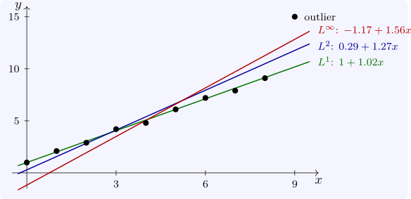
These give linear programming formulations of data fitting. Fitting \(y \approx a + bx\) to points \((x_i, y_i)\) by least absolute deviations (the \(L^1\) fit) or by minimising the largest deviation (the Chebyshev, or \(L^\infty \), fit) are both linear programmes, while least squares (the \(L^2\) fit) is not, though it has a formula. The three can differ greatly when the data contain an outlier (Figure 1).

xy511369oLLL05ut12∞l:::ie 1 0 −r+.2911.+.1072x1.+271.x56x — Figure 1: Three straight-line fits to ten points, the last an outlier. The least-absolute-deviations (\(L^1\)) fit, a linear programme, passes through the bulk of the data and ignores the outlier; least squares (\(L^2\)) is pulled towards it; the minimax (\(L^\infty \)) fit, also a linear programme, is pulled furthest, since it balances the largest deviations (Software 1.4.3).

[next] [prev] [prev-tail] [front] [up]

Questions on this section

Stuck on something here? Ask below and it stays attached to this topic.