8.3 The Theil–Sen Slope

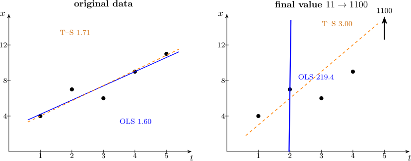
Mann–Kendall says whether there is a trend. It does not say how big it is. The matching estimator is due to Theil and Sen: take the slope between every pair of points and use the median of them.

\[\widehat {\beta } = \operatorname {median}\left \{ \dfrac {x_j - x_i}{t_j - t_i} \ :\ i < j \right \}.\]

There are \(\binom {n}{2}\) such pairwise slopes. Because the estimator is a median, it has a breakdown point of about \(29\%\) — roughly three observations in ten can be arbitrarily corrupted before the estimate is destroyed, against a breakdown point of \(0\) for least squares, where a single bad point suffices.

The pairing of Mann–Kendall with Theil–Sen is deliberate: both depend on the data only through pairwise comparisons, so the test and the estimate agree with one another. In particular \(\widehat {\beta }\) and \(S\) always carry the same sign.

tx12345481oOTtx12345481fi1TO2rL2n1LiS–Sa0–SSgl0i1132n.6.7v.01a01a09ll.4 duaeta11 → 1100 — Figure 7: Why rank methods are used on data that may be contaminated. Left: on clean data the Theil–Sen and least-squares fits are almost the same line. Right: one observation is changed from \(11\) to \(1100\) and nothing else. Theil–Sen moves from \(1.71\) to \(3.00\); least squares moves from \(1.60\) to \(219.4\), a factor of \(137\), and is near-vertical on this scale. The Mann–Kendall statistic does not move at all — \(S=8\) before and after — because the corrupted value is still the largest, so no pairwise sign changes.

[next] [prev] [prev-tail] [front] [up]

Questions on this section

Stuck on something here? Ask below and it stays attached to this topic.