7.3 Laplace’s Method
Watson’s lemma handles integrals whose exponential is \(e^{-xt}\). The following handles the general case, in which the exponent has an interior maximum.
Theorem 7.3.1 (Laplace’s method). Let \(h\) be twice continuously differentiable on \([a,b]\) with a unique maximum at an interior point \(c\), where \(h'(c)=0\) and \(h''(c)<0\), and let \(g\) be continuous with \(g(c)\neq 0\). Then \[\int ^{b}_{a}g(t)\,e^{x\,h(t)}\,dt \ \sim \ g(c)\,e^{x\,h(c)}\sqrt {\frac {2\pi }{x\left |h''(c)\right |}} \qquad (x\to \infty ).\]
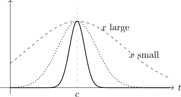
Sketch. For large \(x\) the factor \(e^{xh(t)}\) is overwhelmingly concentrated near \(t=c\). Expanding \(h(t)\approx h(c)+\tfrac 12h''(c)(t-c)^{2}\) and replacing \(g\) by \(g(c)\), \[\int ^{b}_{a}g\,e^{xh}\,dt \approx g(c)e^{xh(c)}\int ^{\infty }_{-\infty } e^{-\frac {x\left |h''(c)\right |}{2}(t-c)^{2}}dt,\] and the Gaussian integral of Section 2.3 evaluates the right-hand side. □
Note 7.3.2. The idea is worth separating from the algebra. As \(x\) grows, the integrand becomes a sharper and sharper spike at the maximum of \(h\), so the integral is determined by an ever-smaller neighbourhood of that point — and in a small enough neighbourhood any smooth function looks like a parabola, which makes the integral Gaussian. The whole method is: find the maximum, fit a parabola, integrate it exactly.
The same reasoning underlies the saddle-point method in the complex plane, and, in statistics, the Laplace approximation to a posterior distribution — which is the statement that a smooth log-likelihood looks quadratic near its maximum, so the posterior looks normal.
Questions on this section
Stuck on something here? Ask below and it stays attached to this topic.