13.3 Implicit schemes

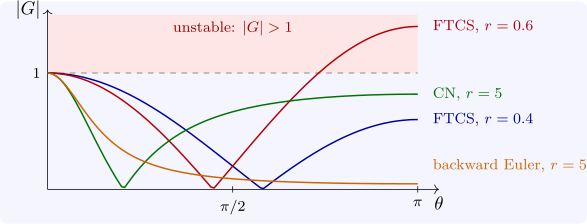
Evaluating the space difference at the new time level gives the backward Euler scheme, and averaging the two levels gives Crank–Nicolson: \[ u_j^{n + 1} - u_j^n = r\,\delta ^2u_j^{n + 1}, \qquad u_j^{n + 1} - u_j^n = \frac r2\bigl (\delta ^2u_j^{n + 1} + \delta ^2u_j^n\bigr ) , \] where \(\delta ^2u_j = u_{j + 1} - 2u_j + u_{j - 1}\). Each step needs the solution of a tridiagonal linear system, which costs only \(O(N)\) operations. Their amplification factors, with \(s = \sin ^2(\theta /2)\), are \[ G_{\mathrm {BE}} = \frac 1{1 + 4rs}, \qquad G_{\mathrm {CN}} = \frac {1 - 2rs}{1 + 2rs} , \] both of modulus at most \(1\) for every \(r\): the schemes are unconditionally stable (Figure 16). Backward Euler is first order in time; Crank–Nicolson is second order, \(O(\Delta t^2 + \Delta x^2)\), and is the standard choice. Its weakness is that for large \(r\) the highest modes have \(G_{\mathrm {CN}} \approx -1\): they are not damped but flip sign at each step, so sharp initial data produce slowly decaying oscillations, which backward Euler, with \(G \to 0\), does not.

𝜃|Gππ1uFCFb∕nTNTac|2stC,CkaS rSwbl,=,ae r rr:=5=d |G E00u|>.6.4ler1, r= 5 — Figure 16: Amplification factors \(|G(\theta )|\) for the heat equation. Low frequencies (\(\theta \) near \(0\)) are treated accurately by every scheme. At high frequencies FTCS with \(r = 0.6\) amplifies, and is unstable; Crank–Nicolson with \(r = 5\) is stable but damps the highest mode only to \(0.82\); backward Euler damps it almost completely.

[next] [prev] [prev-tail] [front] [up]

Questions on this section

Stuck on something here? Ask below and it stays attached to this topic.