9.3 The method of images

Finding \(\varphi ^x\) means solving a Dirichlet problem, so in general \(G\) is no easier to find than \(u\). For regions with symmetry, though, the corrector is the potential of a fictitious image charge placed outside \(\Omega \) so that its field cancels that of the real charge on the boundary.

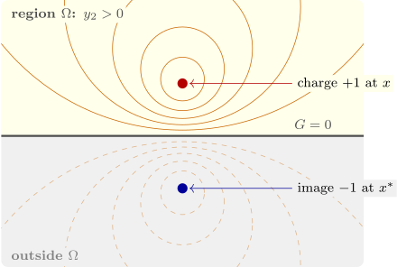
The half-space. For \(\Omega = \{y_n > 0\}\), reflect \(x\) to \(x^* = (x_1, \ldots , x_{n - 1}, -x_n)\). Then \(|y - x| = |y - x^*|\) on the plane \(y_n = 0\), so \[ G(x, y) = \Phi (y - x) - \Phi (y - x^*) \] vanishes there, and \(\Phi (\cdot - x^*)\) is harmonic in \(\Omega \). The Poisson kernel is \(-\partial _{\nu }G = \partial _{y_n}G\) at \(y_n = 0\), which gives \[ u(x) = \frac {x_n}{\pi }\int _{-\infty }^\infty \frac {g(t)\,dt}{(x_1 - t)^2 + x_n^2} \quad (n = 2), \qquad u(x) = \frac {x_3}{2\pi }\int _{\mathbb R^2}\frac {g(y)\,dy}{|x - y|^3} \quad (n = 3) \] for the bounded solution of the Dirichlet problem in the half-plane and half-space. Physically, a point charge \(q\) at height \(h\) above a grounded conducting plane induces on the plane a surface charge whose field, above the plane, is exactly that of a charge \(-q\) at depth \(h\) below it (Figure 12). Its density in three dimensions is \(\sigma = -qh/2\pi (r^2 + h^2)^{3/2}\), and its total is \(-q\) (Software 9.4.2).

Gchimreou=aagtrgis0geeoid −ne+1 Ω1:Ω aatty x x2∗ >0 — Figure 12: The method of images for the half-plane. The level curves of \(G(x, \cdot ) = -\frac 1{2\pi }\log \bigl (|y - x|/|y - x^*|\bigr )\) are the circles of Apollonius on which the distances to the charge and to its image have a fixed ratio. The image charge makes the boundary line one of the level curves, \(G = 0\).

The ball. For the ball \(|y| < a\), use inversion: the image of \(x \neq 0\) is \(x^* = a^2x/|x|^2\), outside the ball on the same ray. For \(|y| = a\) a short computation gives \(|y - x^*| = (a/|x|)\,|y - x|\), so the corrector is the potential of an image of suitable strength at \(x^*\): \[ G(x, y) = \Phi (y - x) - \Phi \Bigl (\frac {|x|}a\,(y - x^*)\Bigr ) . \] In three dimensions this is \(\frac 1{4\pi }\bigl (|y - x|^{-1} - \frac a{|x|}|y - x^*|^{-1}\bigr )\): an image of strength \(a/|x|\). In the plane it is \(-\frac 1{2\pi }\bigl (\log |y - x| - \log (|x||y - x^*|/a)\bigr )\). Differentiating along the radius on \(|y| = a\) gives the Poisson kernels \[ -\partial _\nu G = \frac {a^2 - |x|^2}{2\pi a|x - y|^2} \quad (n = 2), \qquad -\partial _\nu G = \frac {a^2 - |x|^2}{4\pi a|x - y|^3} \quad (n = 3) , \] the first of which is Poisson’s formula of Section 8, found there by Fourier series. At \(x = 0\) the image recedes to infinity and \(G(0, y) = \Phi (y) - \Phi (a)\).

Images work for the heat equation too. On the half-line \(x > 0\) with \(u(0, t) = 0\), the Green’s function is \(\Phi (x - y, t) - \Phi (x + y, t)\), an odd reflection exactly as for the wave equation in Section 4; with an insulated end, \(u_x(0, t) = 0\), the image has the same sign. Wedges whose angle is \(\pi /m\) need \(2m - 1\) images; other regions need other methods, and in the plane, conformal mapping carries the Green’s function of the disc to any simply connected region (Riemann’s mapping theorem).

[next] [prev] [prev-tail] [front] [up]

Questions on this section

Stuck on something here? Ask below and it stays attached to this topic.