12.4 Galerkin’s method and finite elements
The weak form suggests a numerical method. Choose a finite-dimensional subspace \(V_h \subset H^1_0\) and find \(u_h \in V_h\) with \[ (u_h, v)_E = \ell (v) \qquad \text {for all } v \in V_h . \] With a basis \(\phi _1, \ldots , \phi _N\) of \(V_h\) and \(u_h = \sum U_j\phi _j\), this is the linear system \(KU = b\) with stiffness matrix \(K_{ij} = (\phi _i, \phi _j)_E\) and load vector \(b_i = \ell (\phi _i)\). \(K\) is symmetric and positive definite, so the system has exactly one solution.
Theorem 12.4.1 (Céa). The Galerkin solution is the best approximation to \(u\) from \(V_h\) in the energy norm: \(\|u - u_h\|_E = \min _{v \in V_h}\|u - v\|_E\).
Proof. Subtracting the equations for \(u\) and \(u_h\) gives Galerkin orthogonality, \((u - u_h, v)_E = 0\) for all \(v \in V_h\). So \(u_h\) is the orthogonal projection of \(u\) onto \(V_h\) in the energy inner product, and orthogonal projection gives the nearest point. □
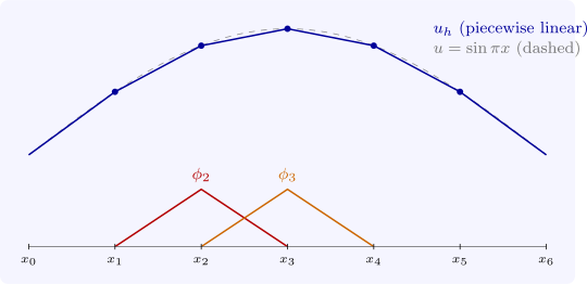
In the finite element method, \(V_h\) consists of continuous piecewise polynomials on a mesh. In one dimension with nodes \(x_i = ih\), the piecewise linear hat functions \(\phi _i\), equal to \(1\) at \(x_i\) and \(0\) at the other nodes, give \(K = \frac 1h\operatorname {tridiag}(-1, 2, -1)\) (Figure 15). Since the interpolant of a smooth \(u\) is within \(O(h)\) of it in the energy norm, Céa’s theorem gives \(\|u - u_h\|_E = O(h)\), and a duality argument (Aubin and Nitsche) gives \(\|u - u_h\|_{L^2} = O(h^2)\). In two and three dimensions the mesh is of triangles or tetrahedra fitted to the region, which is what makes the method so flexible.
Questions on this section
Stuck on something here? Ask below and it stays attached to this topic.