4.6 Examination of Residuals(errors)
The residuals are defined as \(n\) differences \[\widehat {e}_i=Y_i-\widehat {Y}_i,\quad i=1,2,\ldots ,n\] \[\widehat {Y}_i=\sum ^{k-1}_{j=0}X_{ij}\widehat {B}_j\] In performing the regression analysis we make certain assumptions about the errors
- 1.
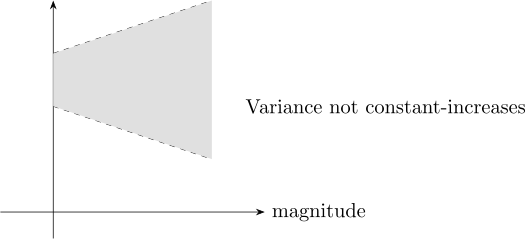
- Constant variance
- 2.
- Normal distribution \(\quad \varepsilon \thicksim ^{iid}N(0,\sigma ^2)\)
- 3.
- Independent
If our fitted model is “correct” the residuals should exhibit tendencies that conform to the
assumptions.
After examining the residuals we must conclude that either the assumptions appear to be violated or
the assumptions do not appear to be violated.
The ways of examining the residuals we will discuss are all graphical the graphical ways are easy to do
are usually very revealing when assumptions are violated.
The four principal way of plotting the residuals are
-
- (a)
- Overall plot (scatter diagram)
- (b)
- In time sequence if order is known
- (c)
- Against the fitted values \(\big (\widehat {Y}\) vs \(\widehat {e}\big )\) \[\widehat {Y}=X\widehat {B}\implies \widehat {e}=Y-\widehat {Y}=Y-X\widehat {B}\] \begin {align*} \widehat {e} & = Y-X\big (X^tX\big )^{-1}X^tY\\ & = \big (I-H\big )Y\quad \text {where}\quad H=X\big (X^tX\big )^{-1}X^t\quad \text {hat matrix} \end {align*}
- (d)
- Against the independent variables \(\big (X_j\) vs \(\widehat {e}\big )\)
In addition to the above four the residuals should be also plotted in anyway that is sensible for a
particular problem under consideration.
The standardised residuals \(r_i=\frac {\widehat {e}_i}{s\sqrt {1-h_{ii}}}\), where \(s=\sqrt {\text {MSE}}\) and \(h_{ii}\) is the \(i^{\text {th}}\) diagonal element of the hat matrix \(H\) \begin {align*} \widehat {e}=\big (I-H\big )Y,\quad Cov\big (\widehat {e}\big ) & = \big (I-H\big )Cov\big (Y\big )\big (I-H\big )^t\\ & = \big (I-H\big )I\sigma ^2\big (I-H\big )^t\\ & = \big (I-H\big )\sigma ^2 \end {align*}
An alternative procedure is to construct a normal plot or half normal plot.
The points should fall approximately on a straight line
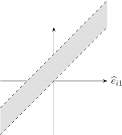
Linear term must be included in the model
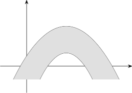
- Linear and Quadratic term should be included
- Need extra terms
- Model transformation of \(Y_i's\)
-
Cross product terms \[\text {i.e}\quad X_jX_{j'}\] \[\beta _0+\beta _1x_1+\beta _2x_2+\beta _3x_1x_2+e\]
\(f_i=\frac {\widehat {e}_i}{\sqrt {\text {MSE}-\big (I-h_{ii}\big )}}\quad \) are known as standardised residuals.
\(\frac {\widehat {e}_i}{\sqrt {I-h_{ii}}}\) are known as standardised residuals.
Questions on this section
Stuck on something here? Ask below and it stays attached to this topic.